Author(s): Ng Kok Wah*, Mimi Fitriana and Thilageswary Arumugam
Structure Equation Modeling (SEM) is a well-known research technique. Before proceed further in data analysis, the researcher describes the fundamentals of Structure Equation Modeling (SEM), as well as its modeling criteria, assumptions, and concepts. The researcher uses Structure Equation Modeling (SEM) to make assumptions about normality, missing data, and sampling errors measurement. In evaluating the model’s fit with the data, Confirmatory Factor Analysis (CFA) starts with a model that anticipates the existence of a predetermined number of latent factors as well as the indicator variables that each factor will load on. Firstly, Normality Test. The “Skewness and Kurtosis” scores of the assessment model, Confirmatory Factor Analysis (CFA), range from -2 to +2. Independent Variables adopted are Self-Efficacy (SE), Perceived Benefits (PB), Behavioural Beliefs (BB), Mediating Variable is Consumer Innovativeness (CI), and Dependent Variable is Health Protective Behaviours (HPB). This study used a total sample size of 400 respondents of private healthcare customers, indicating that the data was normally distributed and satisfied Structure Equation Modeling (SEM)’s normality predictions. Secondly, missing data check. Missing data would jeopardise the statistical analysis in later part and the result might not be able to represent the idea from population. As a result, those questionnaires with more than 30% missing value would be eliminated and excluded from analysis to prevent such phenomena happened. Thirdly, measurement and sampling errors. Minimising sampling error was done by using suitable sample size. A widely used minimum sample size estimation method in PLS-SEM is the “10-times rule” method, which builds on the assumption that the sample size should be greater than 10 times the maximum number of inner or outer model links pointing at any latent variable in the model. Lastly, model fit measures. The study model meets all of the fit indices in general [1].
Modern research tools and techniques facilitate decision making. Initially, the current study concentrates on the Structure Equation Modeling (SEM) research technique. Likewise, Structure Equation Modeling (SEM) is a well-known research technique. Before proceed further in data analysis, the researcher describes the fundamentals of Structure Equation Modeling (SEM), as well as its modeling criteria, assumptions, and concepts. Making decisions is an important task in many aspects of life. Global forces and economic openness drive researchers to implement research-based decisions. Structure Equation Modeling (SEM) establishes the relationship between the measurement model and the structural model based on the theory’s assumptions. It combines Factor Analysis and Linear Regression. Likewise, Regression Models are additive, whereas Structure Equation Models (SEM) are relational in nature, which distinguishes the regression and Structure Equation Modeling (SEM) decision-making approaches. Structure Equation Modeling (SEM) attempts to justify the acceptance or rejection of a proposed hypothesis by examining the direct and indirect effects of mediators on the relationship between an Independent Variable (IV) and a Dependent Variable (DV). Structure Equation Modeling (SEM) also examines the role of controls and moderators. Three characteristics distinguish all Structure Equation Models (SEM) [2-4].
Likewise, the researcher uses Structure Equation Modeling (SEM) to make assumptions about normality, missing data, and sampling errors measurement. In evaluating the model’s fit with the data, Confirmatory Factor Analysis (CFA) starts with a model that anticipates the existence of a predetermined number of latent factors as well as the indicator variables that each factor will load on. After that, the researcher put the model to the test by collecting a sample of respondents from the target population and assessing those variables. The observed associations in the dataset should be well-accounted for by the model if it gives a reasonable approximation. To put it another way, the model needs to offer a strong match to the data. Likewise, the following analysis describes the methods for evaluating the fit of path models to the data. Each of those methods may also be used to evaluate the fit of Confirmatory Factor Analytic (CFA) models. Since Confirmatory Factor Analysis (CFA) models are frequently more complex than route analytic models, a few adjustments will be required, but the fundamental approach to evaluating fit stays the same. Likewise, reviewing significance tests for factor loadings and overall Goodness of Fit Index (GFI) such as SRMR, NFI, Chi-Square and other assessments come first in the procedure. From there, other indices such as R2 values and modification indices are reviewed.
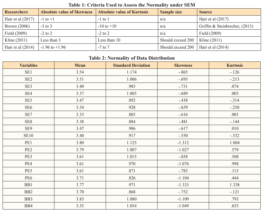
The first and most important assumption before building the model and checking its fit indexes is that the observations are normal. The observations need to come from a normal population that is both continuous and multivariate. However, data normality is a rare occurrence in the real world. As a result, the researchers employ an estimation technique based on the Skewness and Kurtosis of the data at hand [2]. Likewise, if the variable in the study reveals normality, the Maximum Likelihood (ML) approximation technique is used to find parameter estimates. However, if the normality conditions of the data are violated, alternative estimation techniques such as Asymptotic Distribution Free (ADF) are used. Models of moderate size pose a problem for Asymptotic Distribution Free (ADF). With n variables, the formula is u = 1/2 n (n+1). In the case of non-normal data, u represents the elements required to build a model. Therefore, the normality assessment had been executed to analyse whether the data collected is normally distributed or none normally distributed. Likewise, when data are distributed normally, putting them on a result in graph a bell-shaped and symmetrical image is often named as the bell curve. In the distribution of such data, mean, median, and mode are all the same values and coincide with the peak of the curve shape. The most commonly utilised examination to determine normality is shown in Table 1 below. It is recommended as one of the most often used metrics of normality data among all the offered bench-mark measures. As a result, by using “-2” to “2” for Skewness and Kurtosis, the researcher was able to determine the normalcy of data distribution. Likewise, the symmetry of the distribution is measured by skewness, whereas the heaviness of the distribution tails is determined by kurtosis. Skewness is a measure of asymmetry in a probability distribution that differs from the symmetrical normal distribution (Bell curve) in a given collection of data in statistics. The normal distribution aids in determining skewness. Likewise, when the term “normal distribution” is used, it refers to data that is symmetrically distributed. Because all measures with a central tendency lie in the middle, the symmetrical distribution has zero skewness. In other words, when data is symmetrically distributed, the number of observations on the left and right sides are equal. The left- hand side contains 45 observations, and the right-hand side has 45 observations if the dataset has 90 values. The normality of data distribution is shown in Table 2 [2,5,6].
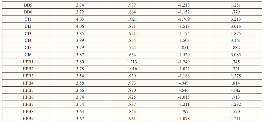
According to Table 2, the “Skewness and Kurtosis” scores of the assessment model, Confirmatory Factor Analysis (CFA), range from -2 to +2. This study used a total sample size of 400 people, indicating that the data was normally distributed and satisfied Structure Equation Modeling (SEM)’s normality predictions. Likewise, the mean of the data is bigger than the median in positively skewed data (a large number of data-pushed on the right-hand side). In other words, the outcomes are skewed to the negative. Because the median is the midpoint value and the mode is frequently the highest, the mean will be higher than the median. As a result, it has been decided to keep all of the details in the structures for further investigation.
Variables in the study should be filled out completely in data forms. There is simply no missing data in any variable. This approach assumes that missing data is completely irrelevant to the study, but this is not the case. Muthen et al. advocate new approach when data is Missing at Random (MAR). Likewise, instead of using pairwise and list-wise deletion to deal with missing data. Later studies revealed that Muthen’s and others’ approach is only applicable when missing data is in small numbers. When using the maximum likelihood technique to estimate the parameters in Structure Equation Modeling (SEM), an imputation approach is available to address the complexities of handling missing data. In sum, missing data might occur when respondents might overlook on certain questions or reluctant to answer those questions. Missing data would jeopardise the statistical analysis in later part and the result might not be able to represent the idea from population. As a result, those questionnaires with more than 30% missing value would be eliminated and excluded from analysis to prevent such phenomena happened [2].
Errors in measurement caused by biassed tools and techniques used for information collection, as well as errors on the part of respondents, affect Model Fit Indexes. Likewise, the standard error is also affected by the variance of the given dataset. The standard error decreases as the variance increases, which violates the assumptions of data normality.emphasised that increasing variance does not affect parameter estimation, but it does affect error approximation. On simulated models with a large number of small factors, the Maximum Likelihood (ML) and Ordinary Least Squares (OLS) estimation techniques were compared, and it was discovered that OLS is a better approximation technique than Maximum Likelihood (ML). This is due to the fact that Ordinary Least Squares (OLS) makes no distribution assumptions.posed a key question on how perfect are the estimations of a model that represents the real world imperfectly? Likewise, previous studies emphasised the importance of pre-tests in dealing with measurement and sampling errors [2,8,7]. In other words, observational error also known as measurement error, it is the difference value between measured value and true value. It was resulted from random error and systematic error. Random error was error caused by surrounding factors and expected in the research. For systematic error, it usually occurred in non-reliable measuring tools, such as low Reliability research instruments. These errors might propagate and result in a big difference of outcome when used for several analysis involving formulae. Hence, there were some steps in reducing measurement error. Firstly, the input raw data into excel were recheck for several times to minimise human error and increase accuracy of the data. Secondly, pilot testing on the research instrument can greatly test the Reliability and accuracy of the instrument. Likewise, those statements in survey that reduce Reliability would be eliminated until the Reliability of research instrument reach optimum level. Then, multiple statements in questionnaires were used to measure same construct in order to minimise random error which beyond the control of researcher. In addition, sampling error might occur when researcher does not select a sample that represent the opinions from targeted population. As a result, the analysis of research does not represent the whole idea of entire population. The result might deviate from true population value because sample was an approximation drawn from entire population. As a result, minimising sampling error was done by using suitable sample size. A widely used minimum sample size estimation method in PLS-SEM is the “10-times rule” method, which builds on the assumption that the sample size should be greater than 10 times the maximum number of inner or outer model links pointing at any latent variable in the model [1].
A structural model should also be analysed in relation to substantive theory, even though fit indicators are a useful guide. It departs from the initial goal of Structural Equation Modelling (SEM), which was to test theories, by letting model fit guide the research process [9]. In addition, Fit Indices could suggest that a model fits well whereas, in reality, some of its components may not [9-11]. In fact, the topic of Fit Indices “Rules of Thumb” is very current right now, with some industry professionals pushing for a total abandonment of Fit Indices [9]. There have been a few fit metrics used in the past literature to measure Structural Model Fitness using PLS-SEM. To assess fit measures, the researcher uses “Standardised Root Mean Squared Residual” (SRMR), exact fit criteria like “d_ULS”, “d_G,”, “Chi-Square”, “NFI”, and “RMS_theta”. The structural model fit measures are shown in Table 3.
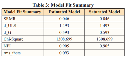
Likewise, the model is judged to be a good match when the Standardized Root Mean Squared Residual (SRMR) is less than or equal to 0.08 [12]. The Standardized Root Mean Squared Residual (SRMR) of this research model is 0.046, as given in Table 3, indicating that it is well-fitting. In finding the exact fit of the model, the squared Euclidean distance (d ULS) and the geodesic distance (d G) are two (2) crucial criteria. Likewise, the difference between d ULS and d G should be non-significant (p-value > 0.05) with a confidence interval of 95 percent and 99 percent for the model to fit effectively [13]. The p-value for 1.493 in the estimated model is 0.824 at the 95 percent confidence interval and 0.902 at the 99 percent confidence interval, respectively. The p-value for 0.593 in the estimated model is 0.399 at the 95 percent confidence interval and 0.421 at the 99 percent confidence interval, respectively. The gap between “d_ULS” and “d_G” in the estimated and saturated models is not substantial, as seen in Table 3. As a result, the model is well-established. In terms of the Normed Fit Index (NFI), the model fit value is estimated using chi-square values [2]. The greater the fit, the closer the NFI is to 1. Likewise, the NFI value for the calculated and saturated model in this research model is 0.905, which is close to 1. It denotes that the model is a good match. The “rms-Theta” was used to perform more model fit analysis. According to Henseler et. al. “rms Theta” values less than 0.12 indicate a good fit model, while any value larger than 0.12 indicates a poor fit model. The underlying research model is regarded a good fit model because the “rms Theta” value is 0.093, which is less than the threshold value of 0.12. Likewise, the study model meets all of the fit indices in general. Furthermore, model fit indices like Standardized Root Mean Squared Residual “SRMR,” “d ULS,” and “d G,” as well as “rms Theta,” ensured that the existing structural model is fit enough to measure the build of the study model. As a result, the existing research structural model is adequate for measuring the current research build. Those statistics and indices can be used to evaluate model fit [12].
In addition, Goodness of Fit Index (GFI) is also one of a statistical method with the Chi-square to Degrees of Freedom (DF) ratio and Root Mean Squared Error (RMSE). Goodness of Fit Index (GFI) values lie between 0 and 1, where values of 0.10 (small),0.25 (medium), and 0.36 (large) indicate the global validation of the path model. Likewise, the ratio of the Goodness of Fit Index (GFI) less than or equal to three determines a model fit as well, and between 2.0 and 5.0 is acceptable model fit requirements [14]. In analysing the performance of both the measurement and structural models, Goodness of Fit Index (GFI) can be utilised to estimate the total prediction power of the big complex model. According to Hussain et. al., 0.1 indicates a little explanation of the model, 0.25 indicates a medium (big) explanation, and 0.36 indicates a large explanation of empirical data, implying that the path model is globally validated. A good model fit, according to, demonstrates that a model is frugal and acceptable. Also, Goodness of Fit Index (GFI) is well-defined as the geometric mean of the Average Variance Extracted (AVE) and Average R² for endogenous construct [15]. Likewise, the following formula is proposed to calculate the Goodness of Fit Index (GFI) from the Table 4 below, Goodness of Fit Index (GFI)= √ (Average R² x Average Communality).
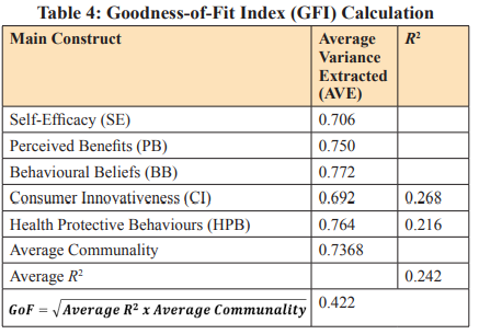
Referring to Table 4, The Goodness of Fit Index (GFI) for this study model was estimated as 0.268. Table 4 above indicates that the empirical data fits the model satisfactorily and has a significant predictive potential in contrast to the baseline values, since 0.422 above the threshold value of 0.36. To summarise, before developing a model to test the proposed hypothesis, the researcher needs to consider the assumptions and concepts of Structure Equation Modeling (SEM). Likewise, Structure Equation Modeling (SEM) is more or less an evolving technique in the research, which is expanding to new fields. Furthermore, it provides new insights to researchers for conducting longitudinal studies [2].
Structure Equation Modeling (SEM) establishes the relationship between the measurement model and the structural model based on the theory’s assumptions. It combines Factor Analysis and Linear Regression [2,3]. Likewise, Regression Models are additive, whereas Structure Equation Models (SEM) are relational in nature, which distinguishes the regression and Structure Equation Modeling (SEM) decision-making approaches. Assumptions for Structure Equation Modeling (SEM), Normality of Data Distribution Analysis & Model Fit Measures is important in enabling the researcher to decide if the research can fittingly draw conclusions from the outcomes of analysis. The normality assessment had been executed to analyse whether the data collected is normally distributed or none normally distributed. Likewise, when data are distributed normally, putting them on a result in graph a bell-shaped and symmetrical image is often named as the bell curve. A structural model should also be analysed in relation to substantive theory, even though fit indicators are a useful guide. It departs from the initial goal of Structural Equation Modelling (SEM), which was to test theories, by letting model fit guide the research process [9]. In addition, Fit Indices could suggest that a model fits well whereas, in reality, some of its components may not [7,9-12]. Goodness of Fit Index (GFI) is also one of a statistical method with the Chi-square to Degrees of Freedom (DF) ratio and Root Mean Squared Error (RMSE). In other words, future researchers need to constantly discover key techniques to assist decision makers and solve problems [16,17].
The present research was made possible by the guidance, advice and support from supervisor, parents, and friends.