Author(s): Aditya Lakshminarasimhan
In the world of molecular biology, Molecular Docking has become a pillar for understanding complex interactions pivotal for drug design and more. The emergence of sophisticated machine learning models, such as Diffusion Generative Models, have significantly expanded our analytical capabilities. However, this evolution has introduced notable computational challenges. This study aims to examine the trade-off between computational demands and model accuracy. Our methodology, which incorporates free platforms, illuminates methods to conserve computational resources while maintaining nearoptimal accuracy. Our findings suggest that using 30 samples per complex, 15 inference steps, and 4 batch steps improves pose prediction accuracy and reduces computational resources. The proposed parameters achieve a 14% accuracy increase compared to the 40 samples per complex model and a 56.25% increase compared to the 10 samples per complex model. The optimized inference steps result in a 12.2% accuracy increase over the 20-step control using the 40 samples model and a 24.3% increase using the 10 samples model. Additionally, using 4 batch steps leads to a 40.6% increase in DiffDock Confidence for the 10-sample control and a 0.4% increase for the 40- sample control.
Molecular Docking is a computational technique in the field of Molecular Biology and the Design, Structural Biology, and Biochemical mechanisms and interactions in Biochemistry can be uncovered with the processes of Molecular Docking. Analyzing protein-protein, protein- ligand, and protein-nucleic acid interactions are important case studies especially in the field of Molecular Biology because designing effective drugs that bind to their targets without causing harmful side effects has always been of key importance [1,2].
Successful machine learning approaches, using a wide array of techniques (Diffusion Generative Models and Deep Learning Models), have been proposed to solve this problem of understanding molecular interactions [3-5]. Machine Learning in general, is data and compute intensive. Generative AI Models require even more data and compute given the data processing, embedding layers, and post-processing steps. For example, DiffDock, a Diffusion Generative Model tasked with predicting protein-ligand binding poses, was compiled on 48GB A6000 GPUs [3]. This type of computing power is costly and is often not available.
For this reason, we are interested in analyzing the trade-off between compute and accuracy to make advanced and accurate tools like Generative AI Diffusion models more accessible in medical and lab settings. We investigate this by using free tools like Google Colab. Additionally, we run parameter tests on Number of Samples per given protein-ligand complex, inference steps, and batch size to determine the optimal value of each parameter such that there is an even tradeoff between compute and accuracy. Our findings suggest that using 30 samples per complex, 15 inference steps, and 4 batch steps improves pose prediction accuracy and reduces computational resources. The proposed parameters achieve a 14% accuracy increase compared to the 40 samples per complex model and a 56.25% increase compared to the 10 samples per complex model. The optimized inference steps result in a 12.2% accuracy increase over the 20-step control using the 40 samples model and a 24.3% increase using the 10 samples model. Additionally, using 4 batch steps leads to a 40.6% increase in DiffDock Confidence for the 10-sample control and a 0.4% increase for the 40-sample control.
Molecular docking predicts how two molecules orient to form a stable complex, using search algorithms to suggest potential arrangements and scoring functions to rank them [6,7]. Essential for drug discovery, molecules forming stable structures with proteins are potentially more effective. Recently, state-of-the-art Diffusion Models have been employed to forecast these docking structures.
DiffDock, a groundbreaking paper on diffusion, offers a specialized approach to predict protein- ligand docking using diffusion models.
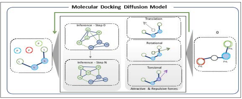
Figure 1: Illustration of the Diffusion Model Adding Perturbations to Generate a Ligand Conformation that can Avoid Steric Clashes in Merging with the Protein. (This Image was Recreated with Inspiration from the Reference [8].
It combines ligand and protein sequences to project their binding combinations while prioritizing the avoidance of steric clashes— overlaps that obstruct binding [3]. To navigate these challenges, DiffDock implements a diffusion process that considers the ligand’s position, orientation, and torsion angles. Through iterative learning from steric clashes, the model successfully guides the ligand to an optimal docking position. Notably, DiffDock achieved a 38% top-1 success rate on PDBBind, surpassing traditional docking at 23% and deep learning methods at 20% [9]. However, its performance demands at least 40 samples as a parameter and a batch size of 10, consuming significant GPU resources and impacting computational speed.
Additionally, EquiBind is introduced as an alternative that employs equivariant diffusion models for molecular binding prediction. Unlike DiffDock, EquiBind uses equivariant techniques to ensure consistent 3D predictions, unaffected by changes in the protein and ligand’s spatial dynamics. This model ensures accurate 3D structures by maintaining ligand bonds and rotations. After its diffusion processes, EquiBind generates a new molecule, showcasing potential in drug discovery.
Diffusion models take a starting visualization and slowly add Gaussian Noise with every iteration. Each time, the model is trained to learn what features were lost until the image is finally nothing but noise. Then, a denoising function slowly adds back features until the final visualization is complete [10]. Diffusion models demonstrate efficiency through their forward diffusion process, where they systematically introduce noise in a gradual and uniform manner. This entails the incorporation of a random distribution of Gaussian noise for each individual pixel within the image. This poses a major benefit because every pixel is being corrupted with noise and the model gathers information about which features were lost. The result is a realistic representation of the original features of the image. The goal of diffusion models is to generate a visualization that is different from the original but retains the qualitative features that compose the visualization. There are two commonly known types of diffusion models which work upon this framework: DDPM (Denoising Diffusion Probabilistic Models) and Score-based diffusion models [11].
DDPMs (Denoising Diffusion Probabilistic Models) serve as the cornerstone for many of today’s diffusion models, utilizing both forward and backward functions. Initially, an image, taken from a particular data distribution, undergoes changes in the forward diffusion process. Here, gaussian noise is progressively added to images, thereby transitioning them from their original complex distributions to simpler ones [12,13]. By the culmination of this forward process, the image has morphed into pure noise, positioning it aptly for training. During the reverse phase, the model undertakes the task of “denoising” the image. Having learned from the forward process, it reconstructs a new image that, while different, retains qualities and distribution characteristics of the original image. Parallel to this, score-based models address generative learning by leveraging techniques like score matching and Langevin dynamics [14].
Score-based models and DDPMs share similarities in their use of forward and reverse noise functions. However, they differ in data selection and distribution. Specifically, Score-based models use a score function to rank data distributions and employ Langevin dynamics to pick datapoints from these more confined distributions, leading to more precisely generated images [15]. On the other hand, DDPMs utilize a broader distribution. Recognizing the parallels in their image generation methodologies, bridged DDPMs and Score-based models in their notable paper, introducing an innovative approach that perturbs data through continuously evolving distributions. This method is dictated by fixed Stochastic Differential Equations (SDE), diverging from traditional finite noise distributions [16]. When this process is inverted, it produces new sample images. A key strength of these models is their capacity to uniformly introduce noise, which is adaptable to both 2D and 3D visualizations. For instance, in a 3D environment, each atom is corrupted with noise, akin to pixels in 2D images. This flexible framework has potential applications in fields such as molecular docking and simulation.
While these diffusion models present a novel generative AI method to solving pressing problems in biochemistry as a larger field, existing models use large amounts of computing resources from GPUs to simulators capable of running multiple protein complexes. For example, the DiffDock model was trained on a variety of ligand and protein poses from the protein data bank [3]. These models were then processed to make presentation-ready data. Given that this Protein Data Bank dataset uses 3d models that need to be simulated in 3d and then processed upon, large amounts of RAM and Disk space are used. This poses an inconvenience for the average hospital or lab which need resources like these for drug design [17].
We propose an experimental study for achieving the high accuracy of DiffDock while using fewer computing resources like RAM and Disk space. To achieve this, we performed benchmark tests to evaluate what features can be reduced while not harshly impacting the model’s accuracy. The DiffDock-Colab model provides 16 parameters to modify, including protein_ligand_csv, complex_ name, protein_path, protein_sequence, ligand_description, out_dir, save_visualization, samples_per_complex, model_dir, ckpt, confidence_model_dir, confidence_ckpt, batch_size, no_ final_step_noise, inference_steps, and actual_steps. Many of the aforementioned parameters are related to file specificity and may not directly affect the protein-ligand pose prediction. Additionally, parameters such as no_final_step_noise and ckpt are internally used in DiffDock to feed information into the Diffusion process during Training. Comparatively, modifying number of samples, inference steps, and batch size are the default parameters suggested to be modified by DiffDock-Colab, and directly impact the volume of poses and accuracy of pose prediction. DiffDock has been trained using 20 inference steps and has two models for Number of Samples. One model uses 10 samples per pose to achieve a 35% top-1 accuracy <2 Angstroms and the other, uses 40 samples per pose to achieve a 38.2% top-1 accuracy <2 Angstroms. While using a 10 samples-per-pose model may seem to be optimal due to only a 3.2% increase in accuracy, these marginal differences can cause the binding affinity to drastically vary [3].
For the context of improving computational runtime while maintaining a favorable accuracy, the focus of this work was on the Interface side of DiffDock rather than modifying the trained model. As such, the pretrained DiffDock model that achieved state- of-the-art accuracy was used, and the interface in Google-Colab was modified through Inference Steps, Number of Samples per complex, and Batch Steps. This framework also allows users from labs to clinics to use this framework for computationally efficient and accurate runtimes. These parameters are the most related to the generated pose between the protein-ligand because, the number of samples per complex adds more processing to generate a higher top 1 RMSD rank value. The number of inference steps represent the number of forward diffusion steps across a given time distribution t. Inference steps are an important parameter to preserve for DiffDock because, when the model is given more forward diffusion steps, it is able to add more random movements (i.e. Steps, Twists, and Turns) which can help the Ligand reach the Protein’s active site without encountering Steric Clashes with the protein. The batch steps also are an important metric to gauge for model performance because, as opposed to inference steps which are primarily used in training, they constitute the number of samples that are processed before the model is updated.
To test the main use-case of DiffDock, single complex docking, we offer single-complex studies. A single complex involves 1 protein and 1 ligand. We hypothesize that using a single complex would offer low compute time and high accuracy. The rationale is that with single-complex docking, the constant number of inference steps in one trial across each sample per complex will allow the ligand to traverse a smaller 3D space of a single protein. For single-complex inference, we tested 6agt and the ligand ‘COc(cc1) ccc1C#N’.
We also performed five trials for each of the parameters – inference steps, number of samples per complex, and batch steps – such that we could ensure variability in confidence is due to number of samples and not by chance. Two of the metrics that we recorded with each trial are DiffDock Confidence prediction and binding affinity. Given that DiffDock uses a unique scoring function ‘DiffDock Confidence’ it is different from past approaches that measure binding affinity. This is namely because of the approach that DiffDock uses. Instead of finding a pocket where binding affinity is the strongest (most negative), it uses a minimized RMSD approach, which seems to be a more efficient and accurate approach compared to previous studies. The Google Colab- DiffDock interface does offer a Binding Affinity prediction through GNINA Minimized scoring function so that each DiffDock pose can be scored. Additionally, DiffDock confidence and correlation with binding affinity has yet to be analyzed based on modifying parameters, so the GNINA minimized binding affinity values were scored for each trial and notated as well. It should be noted, however, that the DiffDock confidence value is scored based on comparison to the true ligand-binding pocket. In the case of scoring predictions, a higher DiffDock confidence value shows a tendency to be more accurate, if the true protein-ligand were experimentally docked.
A single protein-ligand complex was used for evaluation because in the context of simple protein- ligand docking, a protein-ligand pair is benchmarked against various iterations of the same complex. That is, the aim of DiffDock is to predict the positioning of the ligand within the Protein. By electing one protein-ligand complex, modifying parameters, and comparing that complex to itself, a framework can be achieved for improving DiffDock prediction for other complexes. Given that this work aims to identify a trade-off between the number of samples that can be used for a given protein while maintaining reasonable compute resources, this framework offers an optimal number of samples per complex, such that a combination can be met for other protein-ligands as well. Naturally, one unique protein-ligand complex will vary from another in terms of confidence (scored by the scoring function). As such, the confidence prediction for number of samples in one complex is incremented and compared to the same complex. While the confidence values will vary, drastically in some scenarios, between thousands of protein-ligand complexes, the trend in confidence will remain similar because the accuracy and compute time of one single protein-ligand complex is being compared to the same protein-ligand complex under different parameter values to gauge this tradeoff.
Similarly, with regards to inference steps, the protein-ligand complex for 10 inference steps is compared to the protein-ligand complex for 20 inference steps. The comparisons established in this study are against the same protein-ligand complex under different parameter values.
Control groups were defined as the parameters used by DiffDock: 10 samples per complex, 40 samples per complex, 20 inference steps, and 6 batch steps. When modifying the number of samples, the other two parameters were set as control groups, 20 inference steps and 6 batch steps were used. When modifying the number of inference steps, batch steps were set to 6 steps for two scenarios: 10 samples per complex and 40 samples per complex – the control groups were established based on DiffDock’s two major models. When modifying the batch steps, the number of inference steps was set to 20 (default) for two scenarios: 10 samples and 40 samples.
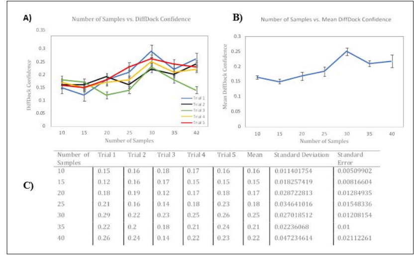
Figure 2: Side-by-Side Panels of Modifying Number of Samples and Effects on DiffDock-Predicted Confidence. Panel A) represents the effects of changing the Number of Samples on DiffDock- Predicted Confidence for Five Trials. The horizontal axis represents the Number of Samples, and the vertical axis represents DiffDock- Confidence. DiffDock Confidence is an index for the relative accuracy of a DiffDock Prediction and isn’t measured in units. Error Bars, representing Standard Error of the Mean, are shown for each Trial. Panel B) represents the effects of changing the Number of Samples on the Mean DiffDock Confidence across all Five Trials. Standard Error of the Mean Bars are shown for each Mean Trial Datapoint. Panel C) is a data table with the DiffDock- predicted Confidence metrics for each Trial and Mean. Standard Deviation and Standard Error of the Mean values are provided. Each trial was conducted using the 6agt protein and “COc(cc1) ccc1C#N” ligand.
To test the effect of changing the Number of Samples on DiffDock predicted Confidence, Google- Colab was used, and both GPU and CPU times were tested. In Panel 2A) 5 trials were conducted, with each trial containing 7 simulations. Each simulation is an increment in 5 samples. In Panel 2A) the general trend for Trials 1, 2, 4, and 5 is an increase in DiffDock-Predicted Confidence, with the exception for Trial 3. While there is a general upward trend in each of the Trials mentioned, there seems to be a clear spike at 30 samples per complex. When tested on CPU, the run- time for 30 samples per complex was 10 minutes and used 55% of the RAM offered by Google-Colab. When tested on the T4 Google-Colab GPU, the run-time for 30 samples per complex was 4 minutes. Despite DiffDock Results suggesting its highest accuracy for the 40
Samples-per-complex method compared to 10-samples-per- complex, this Panel may suggest that using 30 samples per complex can increase DiffDock Confidence to the true ligand position within the protein. Panel 2A) and Panel 2B) do suggest, however, that using 40 samples per complex uses more computing resources and lowers the accuracy of the DiffDock-Predicted Poses.
To first test whether the differences in DiffDock confidences in each Trial were statistically significant, a one-way ANOVA Test was conducted. The mean of each Trial was collected and the overall mean of all data in all trials was conducted.
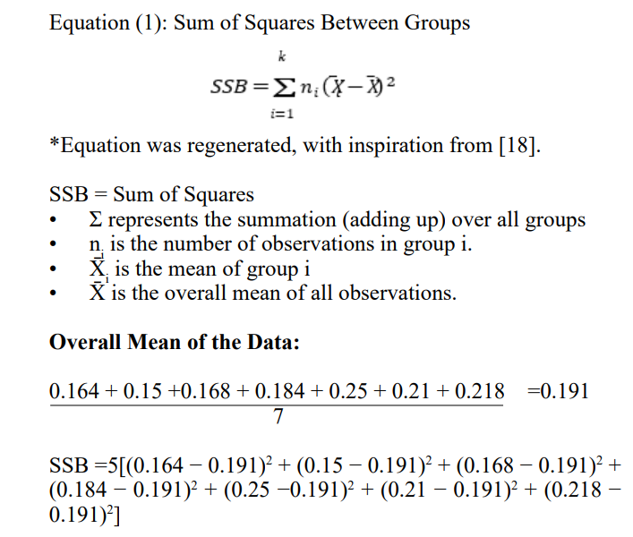
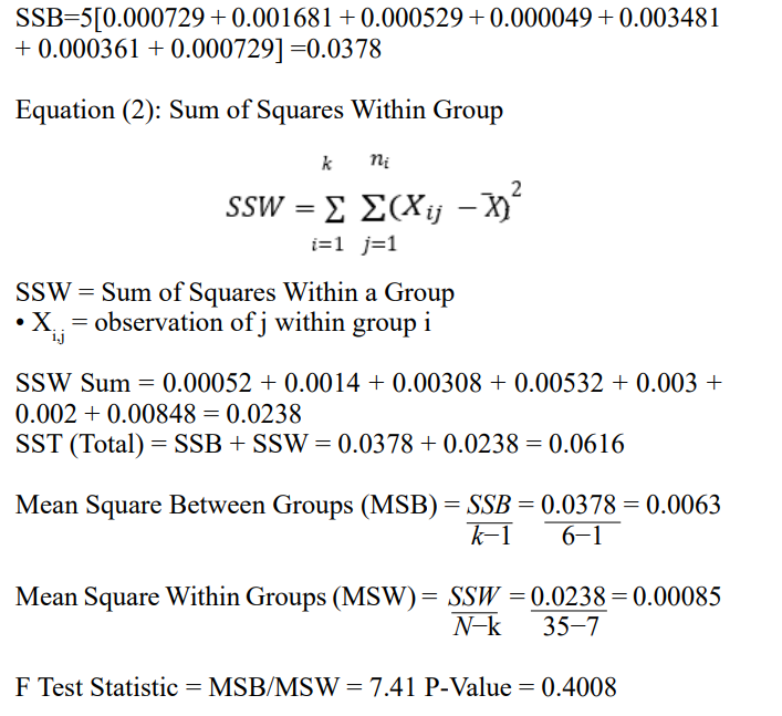
Considering that the P-Value of 0.4008 > α=0.05, 0.01 or any statistically reasonable significance level, it can be said that there is no statistically significant difference between each of the DiffDock Confidence values generated in Trials 1 through 5, and any difference in the trials is due to chance.
In Panel 2B) the Standard Error bars for each number of samples/ DiffDock confidence are shown. Using 30 samples per complex is Statistically Significant compared to using 10, 15, 20, 25, and 35 Samples per complex. The error bars do overlap with using 40 Samples per complex, indicating that the results were not statistically significant. It can still be noted, however, that the majority of trials indicate that using 30 samples per complex is more accurate and uses less compute than using 40 samples per complex. As such, using 30 samples per complex would not only yield a better ligand-protein pose, on average, but also use less compute resources.

Figure 3: Effect of Modifying Number of Samples on GNINA Binding Affinity. As the Number of Samples were Modified, the Respective GNINA Binding Affinity was Calculated per Top-1 Sample. Each Trial was Conducted using the 6agt Protein and “COc(cc1)ccc1C#N” ligand
As seen in Figure 3, the GNINA Binding Affinity varies with no specific trend. Despite Figure 2A) and 2B) suggesting that using 30 samples per complex causes a statistically significant improvement to DiffDock Confidence, the binding Affinity doesn’t change. This is because, the Binding Affinity is calculated based on Free Energy and positioning of the ligand in respect to its intermolecular attractions to surrounding residues. Additionally, even when the number of samples was modified, the ligand was still docked in the same docking site. This marginal movement within the binding pocket can provide a reasonable consistency of Binding affinity but differences within DiffDock confidence. Considering that the DiffDock predicted poses are designed to dock a protein to a ligand and compare those ligand poses to how the experimental structure would have looked, DiffDock confidence includes more specificity than GNINA Binding Affinity and varies by a larger extent. These results do suggest that there is a discrepancy to how an increasing trend in DiffDock confidence may not correlate to an increase in Binding Affinity, as previously hypothesized.
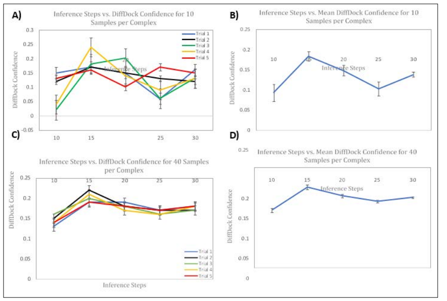
Figure 4: Side-by-Side Panels of Modifying Number of Inference Steps on DiffDock-Predicted Confidence. Panel
A) represents the effects of changing the Number of Inference Steps on DiffDock-Predicted Confidence for Five Trials using 10 samples per complex. Panel B) represents the effects of changing the Number of Inference Steps on the Mean DiffDock Confidence across all Five Trials using 10 samples per complex. Panel C) represents the effects of changing the Number of Inference Steps on DiffDock-Predicted Confidence for Five Trials using 40 samples per complex. Panel D) represents the effects of changing the Number of Inference Steps on the Mean DiffDock Confidence across all Five Trials using 40 samples per Error Bars, representing Standard Error of the Mean, are shown for each Trial. The Horizontal Axis represents Number of Inference Steps, and the Vertical Axis represents DiffDock-Confidence. DiffDock Confidence is an index for the relative accuracy of a DiffDock Prediction and isn’t measured in units. Each trial was conducted using the 6agt protein and “COc(cc1)ccc1C#N” ligand.
We tested the effect of changing the number of Inference Steps on the DiffDock Confidence Values. The metrics calculated in Panels 4A), 4B), 4C) and 4D) were gauged on two scenarios: 10 samples per complex and 40 samples per complex. In DiffDock, the two sets of samples per complex were used to baseline DiffDock predictions to previous efforts. As such, both groups were used to maintain consistency from the DiffDock paper. Five trials were conducted for both scenarios to ensure consistency in the experimental units. A batch size of 6 steps was used, as used in the DiffDock training process and scoring process for testing. Increments of 5 inference steps were used from 10 inference steps to 30 inference steps.
Similar to the number of Samples per complex, another ANOVA test was conducted for Panel
A) and Panel C) to see if the difference in trials was statistically
Using Equation (1) and Equation (2) to perform the ANOVA test for 10 samples per complex, the F Test Statistic was 0.16301 and the P-Value was 0.95463. Considering that the P-Value of 0.95463 > α=0.05, 0.01 or any statistically reasonable significance level, it can be said that there is no statistically significant difference between each of the DiffDock Confidence values generated in Trials 1 through 5, and any difference is due to chance. A similar ANOVA test was conducted for 40 samples per complex. The F Test Statistic was 0.065134, and the P-Value was 0.99158. Considering that the P-Value of 0.99158 > α=0.05, 0.01 or any statistically reasonable significance level, it can be said that there is no statistically significant difference between each of the DiffDock Confidence values generated in Trials 1 through 5, and any difference is due to chance.
In Panel 4A), the trials varied, but generally followed a trend of increasing in DiffDock Confidence from 10 to 15 inference steps and then plateauing or showing no statistically significant difference from then on. In Panel 4B) the mean DiffDock Confidence reveals that using 15 inference steps is statistically significant and performs higher on average than the other choices of inference steps. Despite the effect of the DiffDock confidence with 15 inference steps in Trial 4 being statistically significant in pulling the mean of the DiffDock confidence for 15 inference steps across all trials, the error bars indicate that, on average, the DiffDock confidence from 15 inference steps yields a higher accuracy and uses less compute. In Panel 4C) the trials exhibited far less variability. This is because more samples per complex are used, feeding the reverse diffusion process with more samples before arriving at a Top-1 score. As such, the ligand and its degrees of freedom can be modified and measured with more certainty under the 40- sample model than the 10-sample model. Still, using 15 inference steps was statistically significant and more accurate under each trial. In Panel 4D) this trend is more apparent. With smaller distribution across the trials for a given DiffDock score, 15 inference steps remains to provide more accuracy and compile faster.
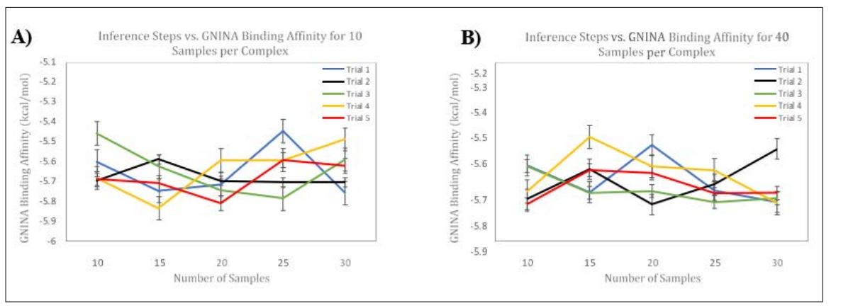
Figure 5: Side-by-Side Panels of Modifying Number of Inference Steps on GNINA Binding Affinity. Panel A) Represents the Effects of Changing the Number of Inference Steps on Binding Affinity (kcal/mol) for Five Trials using 10 Samples per Complex. Panel B) Represents the Effects of Changing the Number of Inference Steps on Binding Affinity (kcal/mol) for Five Trials using 40 samples per complex. Error Bars, representing Standard Error of the Mean, are shown for each Trial. The Horizontal Axis represents Number of Inference Steps, and the Vertical Axis represents Binding Affinity. Each trial was conducted using the 6agt protein and “COc(cc1) ccc1C#N” ligand.
We measured the GNINA Binding Affinity per Top-1 Pose while modifying inference steps for the 10-sample-per-complex model and the 40-sample-per-complex model. While the DiffDock confidence changed with a noticeable trend for both models, the binding affinity did not change with a particular trend, as shown in Figure 5. This finding further suggests that increasing the number of inference steps which changes the gaussian noise per ligand does not statistically affect the binding affinity. Regardless, it seems that DiffDock confidence is a more specific metric due to its ‘confidence’ to the true protein-ligand pose. Whereas, using Binding affinity to score the poses suggests allows for accurate measurement of binding affinity within a binding pocket in a given protein.
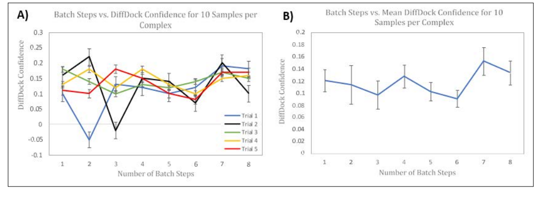
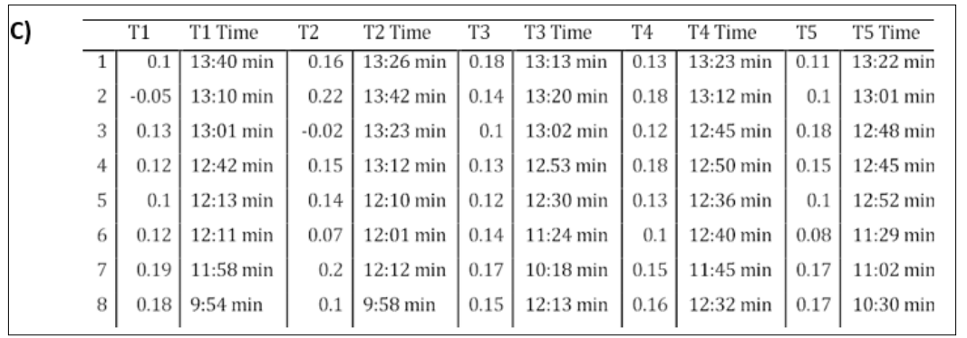
Figure 6: Side-by-side Panels of Modifying Number of Batch Steps on DiffDock Confidence. Panel A) represents the effects of changing the Number of Batch Steps on DiffDock Confidence for Five Trials using 10 samples per complex. Panel B) represents the effects of changing the Number of Batch Steps on the Mean DiffDock Confidence across all Five Trials using 10 samples per complex. Error Bars, representing Standard Error of the Mean, are shown for each Trial. The Horizontal Axis represents Number of Batch Steps, and the Vertical Axis represents DiffDock Confidence. Each trial was conducted using the 6agt protein and “COc(cc1) ccc1C#N” ligand. Panel C) is a table containing all of the data for the 5 trials and includes the runtimes for each inference.
We tested the effect of changing the number of Batch steps on the DiffDock Confidence and GNINA Binding Affinity. In Panel 6A) 5 trials were conducted with 20 Inference Steps and 10 Samples per complex as a control. In each trial, Batch steps were incremented from 1 through 8 steps. Once a batch size of 9 is used, the Google Colab CUDA Out of memory is triggered and the model does not compile. This is because Batch Steps refers to the number of samples that are processed in each ‘batch’. Using a larger batch size can allow the model to compile fast, at the cost of memory. In addition, the Google Colab usage limits are dependent on the rate of usage or memory usage. As such, the limits run out much quicker and allow for less simulations overall, compared to using a smaller batch size and compiling. As seen in Panel 6A) and Panel 6B) there is no specific trend or pattern when changing the number of Batch Steps on DiffDock Confidence. Additionally, as shown in Panel 6C) the general trend decreases in Runtime as batch size is increases. Ultimately, using a batch size of 4 in Panel 6A) is more consistent across the trials and uses 24% of the Memory when compiling. While using a batch size of 7 is more accurate on average, its improved accuracy is not statistically significant and uses 65% of memory. In this case, using a smaller batch step size is more favorable, as it uses less computational resources. As seen in the previous experiments, the batch size did not significantly alter the Binding Affinity predicted by GNINA for the top-1 samples. The range was from -5.391 kcal/mol to -6.082 kcal/mol. The 1st quartile, median, and third quartile were -5.513 kcal/mol, - 5.681 kcal/mol, and –5.757 kcal/mol, respectively.
Using Equation (1) and Equation (2) to perform the ANOVA test for 10 samples per complex, the F Test Statistic was 0.469 and the P-Value was 0.758. Considering that the P-Value of 0.758 > α=0.05, 0.01 or any statistically reasonable significance level, it can be said that there is no statistically significant difference between each of the DiffDock Confidence values generated in Trials 1 through 5, and any difference is due to chance.
To test for whether this pattern existed in the 10 samples per complex set, we also tested this using 40 samples per complex.
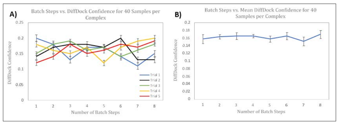
Figure 7: Side-by-side Panels of Modifying Number of Batch Steps on DiffDock Confidence. Panel A) represents the effects of changing the Number of Batch Steps on DiffDock Confidence for Five Trials using 40 samples per complex. Panel B) represents the effects of changing the Number of Batch Steps on the Mean DiffDock Confidence across all Five Trials using 40 samples per complex. Error Bars, representing Standard Error of the Mean, are shown for each Trial. The Horizontal Axis represents Number of Batch Steps, and the Vertical Axis represents DiffDock Confidence. Each trial was conducted using the 6agt protein and “COc(cc1) ccc1C#N” ligand.
As seen in Panel 7A) and Panel 7B), using 40 samples per complex did not cause a significant difference from using 10 samples per complex. Especially in Panel 7B), on average, the number of batch steps is not statistically different from one size to another. Still, using 4 batch steps has a smaller margin of error and is more consistent. As seen in the previous experiments, the batch size did not significantly alter the Binding Affinity predicted by GNINA for the top-1 samples.
The range was from -5.223 kcal/mol to -5.871 kcal/mol. The 1st quartile, median, and third quartile were -5.434 kcal/mol, -5. kcal/ mol, and –5.716 kcal/mol, respectively.
A similar ANOVA test was conducted for 40 samples per complex. The F Test Statistic was 0.265, and the P-Value was 0.898. Considering that the P-Value of 0.898 > α=0.05, 0.01 or any statistically reasonable significance level, it can be said that there is no statistically significant difference between each of the DiffDock Confidence values generated in Trials 1 through 5, and any difference is due to chance.
Overall, the differences observed in modifying batch steps has an effect on the accuracy as noted earlier, however, the more impactful differences would be measured when retraining the DiffDock model to use 4 batch steps instead of 6 batch steps [19-21].
As recent applications in Protein design and Protein interactions continue to be fueled by technological progress, implementing a cautious balance such that the computational cost is still feasible for small labs and clinics. Despite recent attention and advancements in Diffusion Models like DiffDock, a study on the parameters and the relative accuracy that each metric provides is yet to be studied. In this study, we tested the number of samples, inference steps, and batch steps to arrive at an optimal number of each parameter. We conclude that using 30 samples per complex, 15 inference steps, and 4 batch steps not only improves the accuracy of the pose predictions, but also incurs fewer computational resources. On average, the proposed number of samples had a 14% increase in accuracy compared to the 40 sample per complex model and 56.25% increase in accuracy compared to the 10 sample per complex model; The proposed inference steps had a 12.2% increase in accuracy compared to the 20-step control using the 40 sample per complex model and 24.3% increase in accuracy compared to the 20-step control using the 10 sample per complex model; Finally, on average, using 4 batch steps lead to a 40.6% increase in DiffDock Confidence for the 10-sample control and a 0.4% increase in DiffDock Confidence for the 40- sample control. For Batch steps, future studies should be conducted on retraining the model with such parameters and testing the accuracy.
With this study’s ability to determine an optimal value for each of the three parameters, it poses useful in the setting of limited compute power. This study, however, can be extended to a specific field in drug discovery: incorporating RNA receptor flexibility. Many viruses from Covid-19 to RSV have RNA viral signatures. When these signatures bind to cellular receptors, the viral DNA is transmitted. Extending diffusion models to predicting conformations between RNA Viral spike proteins and cellular receptors with high receptor flexibility could allow better molecular targets to be designed to inhibit spike proteins more efficiently.