Author(s): Fatbardha Maloku*, Besnik Maloku and Akansha Agarwal Dinesh Kumar
The escalating annual rise in housing prices introduces volatility and uncertainty into the real estate market, underscoring the critical need for accurate price forecasting systems. Predicting house prices accurately remains challenging due to the multitude of influencing factors. This study aims to identify and analyze key determinants affecting house prices, employing two established machine learning models. Through comparative analysis, the research will recommend the most effective model for enhancing the accuracy of house price predictions.
The majority of people today are engaged in the commercial activity of investing. Stocks, bonds, retirement, education, and other choices are widely used as investments. One of the investment forms that people frequently use is the buying of a property. The process is not simple, despite appearances to the contrary. Any real estate project that is purchased or in which an investment is made sometimes necessitates a series of discrete transactions involving numerous parties. As a result, it might be a crucial decision for both households and businesses. The housing market is currently being impacted by high-interest rates, which have raised home prices and affected both the supply and demand for homes. Because of this, it is crucial to examine additional the key metrics or factors that affect home prices. The purpose of this study is to forecast home values using two well-known machine learning models. Using the House Price Prediction dataset, we will investigate and comprehend how different variables may forecast home values. We will learn the impact of different factors like location, size, house quality, condition etc. on the cost of homes. One of the various techniques for determining the value of a home is prediction analysis. We will utilize both linear regression and random forest regression in this study to forecast house prices that take other aspects into account. The knowledge obtained from this research will help customers decide when is the best time to buy a home as well as real estate investors.
As the housing market is prone to volatility and uncertainty, it's critical to figure out which key metrics influence house price predictability. House prices are commonly assumed to be tied to our economy, but is this true? Despite the vast amount of data available, reliable property price projections are lacking.
In this study, we will examine and comprehend how various features might forecast house prices using the House Price Prediction dataset. How do diverse characteristics like location, house size, age, etc. affect the price of houses? The housing market is currently being affected by the high-interest rates, which have boosted home prices and affected both the supply and demand for homes. Analysis of other non-economic factors that affect housing prices is crucial for this reason. When analyzing the price of a property, this analysis will assist buyers and sellers in focusing on some non-economic factors.
This project's primary goal is to develop a Python-based machine learning model that can learn from this data and calculate the cost of a home in any district given all of the other variables in the dataset.
The methodologies used in this project will start by running an explanatory data analysis (EDA). We will continue to prepare the dataset characteristics for use in model predictions and test a few models to predict home prices in this project.
The exploratory data analysis methodology helps us develop task understanding, which in turn provides us with insights on later feature engineering and handling of missing values.
This dataset was made publicly available on Kaggle, a website for data science competitions. To begin the analysis, we extracted the data and put it into our notebook.
The nature of the data and the relationship between the variables should be examined and investigated before creating the prediction models for estimating house prices. After importing the data into the environment, the attributes are then examined, including names, data types, and the number of missing values.
To assess the effectiveness of the final model, the data are divided into a train set and a test set. Additionally, the data should be formatted to make it simple to read and edit. This process should be done for each column and row in the dataset.
After we prepare the data, we then need to decide how we will deal with the missing data. There are many variables with missing values. We attempt to impute the missing data using the following methods:
We may now begin visualizing our data. To examine the distributions, we first plot the histograms for each numerical variable. We are interested in the distributions' skewness or symmetry as well as any other effects.
Correlation between the Explanatory Variables & Target The relationship between these numerical variables and the target will next be examined. As a result, to see the associations between the variables, we generate a correlation matrix and plot scatterplots.
Linear Regression is a machine learning algorithm based on supervised learning. It performs a regression task. Regression models a target prediction value based on independent variables. It is mostly used for finding out the relationship between variables and forecasting [1].
A linear model assumes a linear relationship between the input variables (x) and the single output variable (y). More specifically, that y can be calculated from a linear combination of the input variables (x) [1].
While training the model we are given:
x: input training data (univariate one input variable(parameter))
y: labels to data (supervised learning)
The best line to predict the value of y for a given value of x is fitted to the model during training. By determining the ideal values for the 1 (intercept) and 2 (coefficient of x), the model produces the best regression fit line. Once we find the best θ1 and θ2 values, we get the best fit line. So, when we are finally using our prediction model, it will predict the value of y for the input value of x.
Random Forest Regression is a supervised learning algorithm. This method combines predictions from multiple machine learning algorithms to make a more accurate prediction. A Random Forest is run by constructing several decision trees at the training time and outputting the mean of the classes as the prediction of all the trees. The random Forest Regression model is powerful and accurate. It is a great solution to many problems, including features with non-linear relationships [2].
The steps involved are described thoroughly in the below section.
Identify your Dependent (y) and Independent Variables (X)- Split the Dataset into the Training Set and Test Set-The importance of the training and test split is that the training set contains known output from which the model learns. The model's predictions are then put to the test using the knowledge it gained from the training set.
Training the Random Forest Regression Model on the Whole Dataset - The parameter n estimators create the n number of trees in your random forest, where n is the number, you pass in. We passed 10. With the help of the fit () function, we can train the model and improve accuracy by changing the weights in accordance with the data values. The predict () method is used to make predictions once our model has finished training.
Predicting the Test Set Results-After successfully creating the Random Forest Regression model, we can assess the accuracy by calculating the R².R² score tells how the model is fitted to the data by comparing it to the average line of the dependent variable. When the score is closer to 1, it shows the model performs well, when it is farther away from 1, it indicates that the model is not performing well.
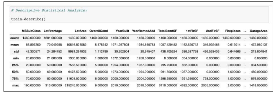
By conducting a descriptive analysis of the data, we will begin solving the house prediction problem. We will learn information from the descriptive analysis of the house prediction data set that is not apparent from a simple glance at the spreadsheet. More information about the house forecast's metadata is provided in the section below.
The house prediction data set's primary columns are summarized as follows:
The data set has a total of 30 columns and 1460 rows. The vast majority of the data set's columns are classified as explanatory variables. The column labeled "Sales Price" will serve as the analysis' predictive variable. We will examine how these explanatory variables or factors affect the prediction of a house's sales price during this analysis. To know more about the statistical values of our dataset, we can use Python functions and methods to gain more insight. In the example below, we've used the describe function to learn more about the count, mean, standard deviation, min, and a max of our data set as well as the summary statistical analysis of the columns in the house price data collection. By doing explanatory data analysis we discover that the maximum sales price for a house is $755,000, the minimum is $349,000 and the average price of a house is approximately $163,000. We can see that there is a total of 30 features or variables, 8 of which are 'objects', 20 of which are 'int64', and 2 which are ‘float64'. According to the documentation of the competition, the variable 'SalePrice', which has a data type of 'int64', is the target or label that we are going to predict.
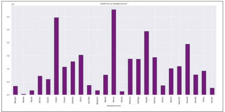
We learned during analysis that the dataset's neighborhood is a key variable. We can observe from the visualization below that the cost of houses varies depending on the neighborhood within the same city. From the visualization, we can notice the diverse distribution of house values among neighborhoods.
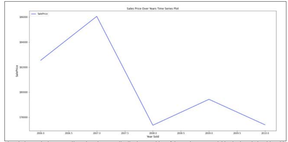
What time of year is ideal for selling a home? According to the analysis from real estate research company ATTOM Data Solutions, late spring and early summer are the greatest seasons of the year to sell a home [3]. However, our house prediction dataset goes a bit more in- depth and shows us the home sales for a period of four years, from 2006 through 2020. From the graph, we can see an increase in the Sales Price in 2007 and a huge decrease in the market in the upcoming year, 2008. We understand that year 2007 had the highest sales prices in the market, whereas in the upcoming year the prices shrank to approximately $8,000.
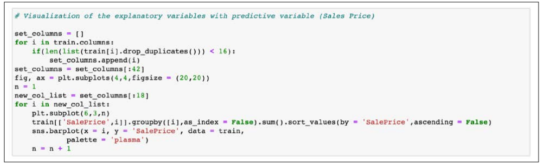
The descriptive analysis comes alive when there are distribution graphics of the explanatory variables in the relationship with the Sales Price predictive variable. In this way, we will get to visualize how our data is distributed before predicting any values. To do that, we have created a function which will go through explanatory columns in the house price dataset and visualize the results.
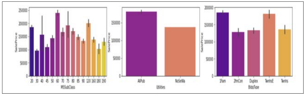
The next set of visuals demonstrates the distribution of MSSubClass, Utilities, and BldgType variables. From the chart, we can see the distribution of our data in different categories. The MSSubClass that has the highest values is the class of 60. The utilities that are highly used are the houses that include all public utilities such as (E, G, W, & S). The building type is approximately distributed the same between single-family houses and townhouse end units.
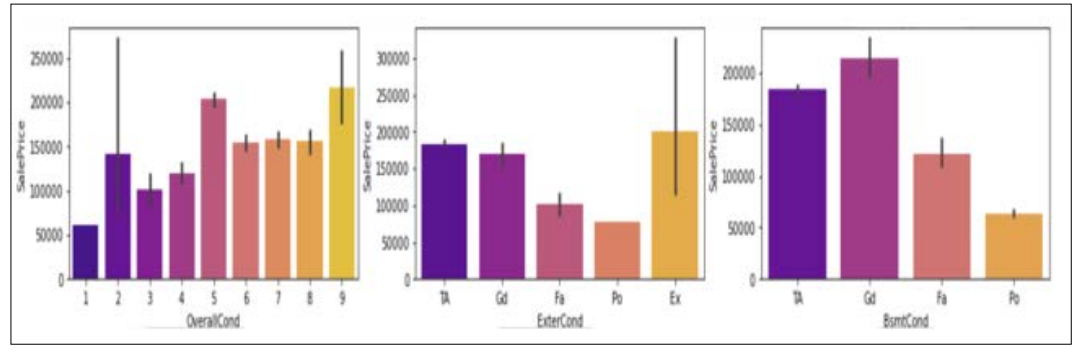
When it comes to the general state of the houses, when the condition of the houses is 9 or above, the sales price of the houses tends to be higher. The exterior condition of the property is crucial, and when it receives top ratings and presents a better impression, the sales price of the home tends to be greater. Conversely, when the exterior condition of the home is poor, the sales price of the home is lower. The general condition of the basement is another factor which plays a high role in the overall sales price of the house.
When the condition of the basement is good then the price of the house tends to be higher than in the houses where the condition of the basement is poor.
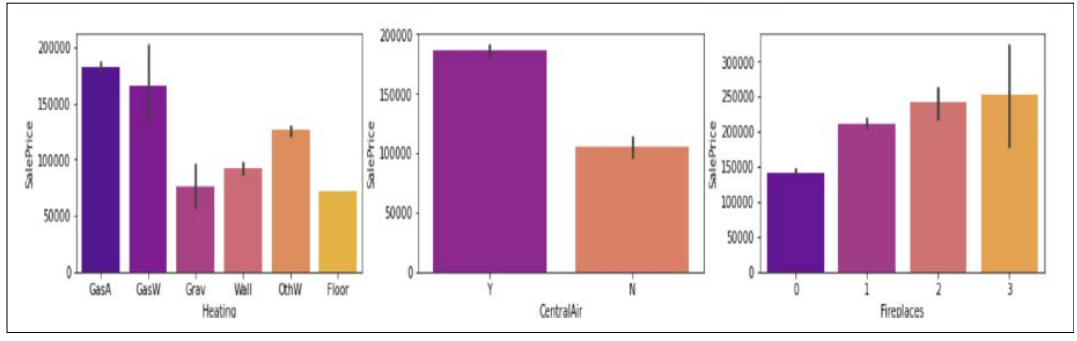
The heating factor is also important. The gas-forced warm air furnace heating option is highly expensive compared to the floor furnace and gravity furnace. The houses tend to be higher in price when the houses contain a central air conditioning system installed in place, versus the ones that don’t. Houses that tend to have a higher number of fireplaces are also more expensive.
The garage and the number of parking spaces are two other factors that consumers consider when purchasing a home. We learned through the analysis that homes with three garages are the most popular among buyers. Additionally, more expensive are homes with 555 square feet of pool space. Don't overlook the importance of the month that the residences were sold.
As we can see, the distribution is quite consistent over the entire month. We noticed a slight difference in the rate of price increases in September.

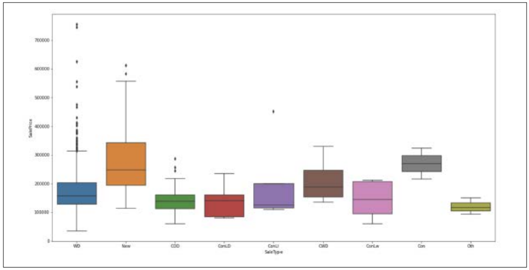
The box plot visualization type can be used to display the distribution of the sales type over the sales price variable. We can observe that the distribution changes between various categories from the graphic below. We can see the category “New” is a category for the houses that are just constructed. This category seems to be higher distributed than the other categories of the types.
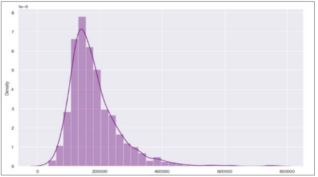
The density distribution of the Sales Price variable is shown in the below graph. The Sales Price target variable has a right-skewed distribution and is not symmetric, which would have an impact on the model, according to the plot below.
Predictive analytics, a subset of artificial intelligence, is a statistics-based technique that data analysts use to formulate hypotheses and analyze past data in order to estimate the chance of a specific future result. Using machine learning and historical data like trends and behaviors, predictive analytics enhances processes. On a set of future data, predictions are made using both predictive analytics and machine learning. In our research, we used machine learning models to predict the possible house price based on the different influential factors which we discussed in the above section.
Before building our machine learning models, we started by running a quick correlation test between variables to identify the highest influencing variables which have a significant effect on house prices. As mentioned earlier, we have considered all the non-economic factors to see which of these influences house prices the most.
Correlation analysis is a test to examine the relationship between the variables in a dataset. With the correlation heatmap and correlation matrix, one can observe the relationship between the explanatory and the response variables. For our study, we used a correlation heatmap to examine the relationship between the variables.
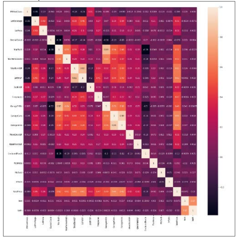
As we can observe from the above heatmap most of the variables have a positive correlation with the sales price which is also known as the house price in our study. Variables like lot area, house condition, basement condition, garage area etc. have a significant relationship with the house prices. We will be taking all of these variables and proceeding to build our machine learning predictive models.
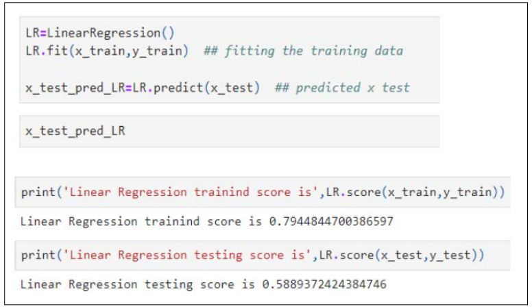
We now move to the most important part of our analysis which is building the machine learning models to predict future outcomes. We used our dataset to train the machine learning models to predict house prices. We started by building the Linear Regression Model and trained it to help predict future outcomes [4].
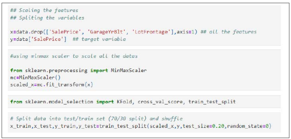
We first used the algorithm to derive our x and y. We removed the garage year built and lot frontage, as these are already covered as a part of the variable house-built year and the square feet of the entire house. We derived the sales price as y and other independent variables as x. We then split the data into train and the test set as 0.80 and 0.20 as shown below.
After deriving the train and test set, we then trained our model and tested the training and testing accuracy. According to the results, the training set has an accuracy of 79.44% as shown below, whereas the testing set accuracy score is 58.89% which is not bad.
To test and see if we can get a better accuracy score with other machine learning models, we decided to use the Random Forest Regressor Model. A random forest is a meta estimator that employs averaging to increase predicted accuracy and reduce overfitting after fitting multiple categorizing decision trees to different subsamples of the dataset.
We used the same split set to build a random forest regressor model and train the model. According to this model results, the training set has an accuracy score of 97.32% and the test set has an accuracy of 82.29% as shown below.
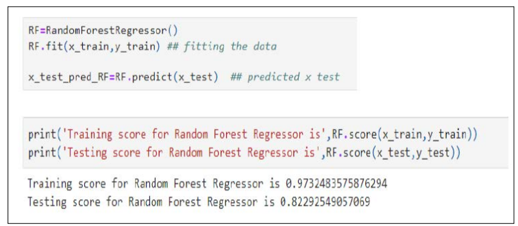
As we can observe, clearly the random forest regressor model is better in comparison with the linear regression model. The reason for achieving a higher accuracy score is to ensure that the predictive outcome is more accurate. Therefore, the random forest regressor model is the clear winner in this case. Further, this trained random forest regressor model can be used to test the dataset which consists of similar variables.
The analysis provided us with a collection of new information. Initially, the data contained both categorical and continuous features, and the target feature had a binary value. The data types for feature values are a mix of int, float, and object. Numerous columns had a significant number of missing values. Most continuous feature variables have outliers, which we dealt with during data pre-processing. Based on the heatmap and plot graphs, there are dependent features that are closely associated with other dependent features. In our analysis, we also noticed the diverse distribution of house values among neighborhoods. When it comes to the general state of the houses, when the condition of the houses is 9 or above, the sales price of the houses tends to be higher.
The exterior condition of the property is crucial. We learned through the analysis that homes with three garages are the most popular among buyers. We noticed a slight difference in the rate of price increases in September. The sales price target variable had a right-skewed distribution which affects the machine learning model.
The machine learning model used in this paper is the linear regression model and the random forest model. We considered all the variables when training our model, except for garage year built and lot frontage as they are already a part of the house build year and the size of the house. We proceeded with all other variables and trained our model, as we saw both the models had a high accuracy score, however, the Random Forest Regressor model had a higher accuracy score with 97.3% for the training set and 82.3% for the testing set, in comparison with the linear regression model with only 79.4% and 58.9% for training and testing, respectively. Therefore, we can conclude that the Random Regression model is the best model for our study which can be used to predict house prices with higher accuracy, given considers the same variables.
For many years, house prices have been interpreted through numerical values that contain various information about the houses. The use of statistical data causes an increase in the number of scientific research based on housing data. One of the frequently studied topics in these scientific studies is the prediction of house prices. Our study is an example of these studies. The house price prediction model uses machine learning algorithms and models. We built two popular machine learning models to train the dataset. We measured their accuracy score on both the training and testing set. Based on the accuracy score, we strongly recommend a random forest regression model for better prediction of house prices.
The model will be able to predict house prices exactly so that buyers or sellers will not get lost. This will be useful to both buyers and sellers as well as real estate agents and companies.
As mentioned above, the Random Forest Regression model has the highest accuracy score in terms of both training and test set. To increase the prediction successes obtained in the study, enrichment can be performed both in the study dataset and in the methods used. Many other variables affect house prices but are not taken into account. Variables such as location, room size, bathroom size etc. that are ignored in most scientific studies can also directly affect the results. For these reasons, instead of using a dataset consisting only of limited variables a large dataset can be used, which also includes variables such as those mentioned here. In addition, there are several other methods which can be used to increase the accuracy and prediction.