Author(s): Barry Setterfield
One key topic in astronomy is the redshift of light from distant galaxies. Currently there are two main models for what is observed, but discrepant data reveal that neither approach gives an adequate answer to the matter. In 1985 a suggestion was made that the answer to this problem may be found in the light emitted from the atoms within the galaxies themselves, rather than something happening to light in transit. That suggestion is examined with a more complete understanding of the vacuum Zero Point Energy (ZPE) that has emerged recently, since, on one view, it controls the electromagnetic properties of space. A review is undertaken of both the redshift and its problems and also the way our understanding of the ZPE has developed. The facts emerging from these reviews are then applied to suggest a different cause for the redshift, and a concordant reason for redshift quantization.
The majority of emitted light comes from atoms as an electron drops from an outer orbit to an inner one. The energy difference between the two orbits is the energy of the emitted photon of light as this image shows in Figure 1 on the top left panel. Alternately, in the reverse process, light is absorbed by an electron when it is elevated from an inner orbit to an outer one. In this case, instead of a bright line on the rainbow spectrum, there is a dark line. If the same two orbits are involved the bright line and the dark line will be in exactly the same position as in the example for hydrogen shown on the two panels on the bottom left in Figure 1. Each element has its own unique differences between its various orbits. This results in something like a barcode of lines on the rainbow spectrum with a pattern which is specific to that element.
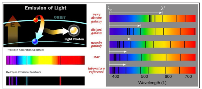
Figure 1: (Left) Production and Types of Spectra. (Right) Redshift of Spectral Lines of Distant Galaxies
However, in the 1920’s something interesting was noted. As we look progressively farther and farther out in space, we are also looking progressively further and further back in time. Some special types of stars have a known luminosity which gives us a very good idea of the distance. It was established in the mid1920’s that, as we look to greater and greater distances (and hence earlier times) in the cosmos, this same unique barcode pattern of lines for any specific element will be shifted as a whole down towards the red end of the rainbow spectrum, as on the right-hand panel in Figure 1. Here the laboratory reference barcode for the element is at the bottom, and the same element emitting light is from galaxies which are more and more distant astronomically as we go towards the top of the panel.
This effect is called the redshift, and is designated “z”. The farther we look out into space, the greater is the redshift of the emitted light and the higher the value of z. As we come closer and closer to our own time and location in space, the emitted light shifts towards the blue end of the spectrum (becomes bluer) until all atomic transitions have the same color or energy as our laboratory standards and so z = 0. In astronomical applications, the redshift may be designated as either “z” or “(1 + z)” and is derived mathematically from the change in wavelength of the observed spectral line divided by the laboratory standard wavelength for that line. In every case, “z” is a dimensionless number (that is just a number without any units, such as meters or centimeters).
The standard explanation for this “redshift,” or longer wavelength for a given line, is that the universe is expanding at an ever-faster rate and so the result is a stretching out of the light waves. This is meant to happen for one of two reasons. The first reason comes from the idea that, as the fabric of space was stretched out, so, too, were the light-waves traveling through space. This resulted in longer wavelengths at the time of reception than at the time of emission, thereby giving a redshift in the wavelength that was originally emitted. The concept is illustrated in Figure 2: The problem is that such a stretching of wavelengths will also stretch or smear out or proportionally broaden the originally sharp spectral lines emitted by the various elements and which appear like a bar-code in spectral images of distant galaxies. It is important to note that the expected broadening or smearing out of spectral lines does not usually occur. For example, see reference [1]. Rather, distant galaxies have spectral lines which are just as clear and sharp as nearby objects, despite a redshift in their wavelengths, as in Figure 2.
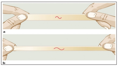
Figure 2: In the top diagram, a wave is drawn on a piece of unstretched elastic fabric. Then in the bottom diagram, the fabric is stretched. As it does so, the wavelength is stretched proportionally. This is how it is proposed that expanding the fabric of space causes the redshift. The problem is that this would also proportionally broaden the black spectral lines of the elements, but they stay thin.
The only other scientifically popular mechanism is to have a static fabric for space-time and galaxies racing away from each other through it (Left in Figure 3, with MW = Milky Way galaxy). This originally was Einstein’s proposal. On this model, the redshift is thought to be due to a Doppler effect. In this effect, light waves coming forward from a moving source ‘bunch up’ ahead of it and are shortened. Light waves moving back from the source trail out behind and are lengthened - giving a redshift. The farther away a galaxy is, the faster it is moving away from us. The faster the motion is away from us, the greater is the redshift. The effect is shown on the right in Figure 3.
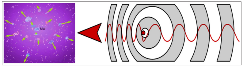
Figure 3: (Left) - Galaxies Racing away from us, being Faster with Distance. (Right) - The Doppler Effect
One problem with this proposal was pointed out by Misner, Thorne and Wheeler in their tome on Gravitation [2]. While discussing quasar redshifts greater than z = 1, they state: “Nor are the quasar redshifts likely to be Doppler; how could so massive an object be accelerated to v ~ 1 [the speed of light] without complete disruption?” [2]. Since the galaxies and quasars involved show no signs of disruption, the conclusion is that the redshift does not have a Doppler origin. From the luminosity measurements the relationship between redshift and distance is fairly secure, but the origin of the redshift itself seems to be more problematic.
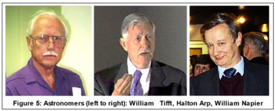
These problems were exacerbated by data that was first noticed in 1976 by William Tifft, the astronomer at Tucson Observatory, Arizona. Tifft published several papers indicating that redshift differences between galaxies in the Coma cluster did not progress smoothly, but were ‘clumped,’ or grouped, and changed in jumps [3]. The study was extended to other galaxy clusters and groups. The effect seemed to be everywhere and became referred to as the quantized redshift [4]. If the redshift were actually due to galaxies racing away from each other, as the Doppler shift interpretation requires, then these speeds of recession should be distributed like those of cars smoothly accelerating on a highway. That is to say, the overall redshift function should be a smooth curve. But the results that Tifft obtained indicated that the redshift measurements jump from one plateau to another like a set of steps. It was as if every car on the highway traveled only at speeds that were multiples of, say, 5 miles per hour, with nothing in between.
On either of the standard models, it was difficult to see how any cosmological expansion of space-time or, alternatively, the recession of galaxies, could go in jumps. Even more puzzling was the fact that some jumps actually occurred within galaxies. If the redshift was indeed due to motion, then a redshift quantum jump going through a galaxy would mean that different halves of the galaxy would be moving at different speeds. This would force the galaxy to disrupt. This is not occurring.
A number of astronomers collected data that supported the quantization concept, but they and the data were both strongly criticized. In 1985, Sulentic and Arp accurately measured the redshifts of over 260 galaxies from more than 80 different groups, and were surprised to discover the quantizations that Tifft and Cocke had found [5]. In an attempt to prove the whole concept wrong, Bruce Guthrie and William Napier of the Royal Observatory, Edinburgh, used the most accurate hydrogen line redshift data available, as well as doing their own measurements and developing rigorous statistical tests. By the end of 1991, 106 spiral galaxies gave a quantization of 37.5 km/s; by November 1992, a further 89 spiral galaxies gave a quantization of 37.2 km/s [6-8]. In 1995 a further 97 spirals showed a 37.5 km/s quantization and they submitted a paper to Astronomy and Astrophysics [9]. The referees asked them to repeat their analysis with another set of galaxies, which Guthrie and Napier did with an additional 117 galaxies. The same 37.5 km/s quantization was in this 1996 data set and the paper was accepted [10]. Samples of their data are plotted in Figure 4.
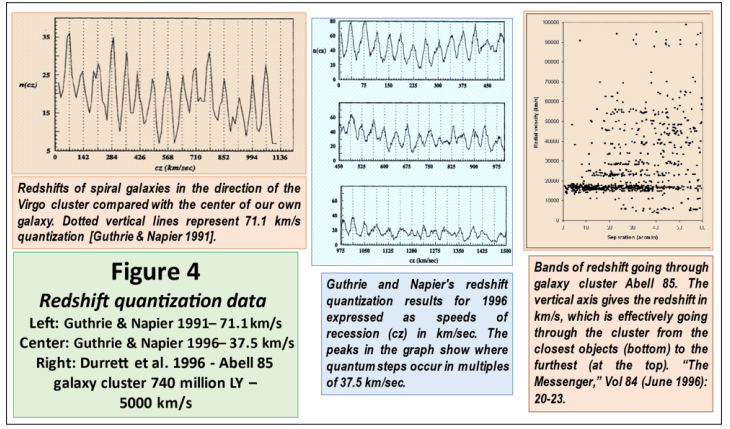
The horizontal axis in Figure 4 is “cz”; in other words, the redshift as a “velocity.” There, the velocity goes from 0 km/s (near our galaxy) up to 1500 km/s (towards the Virgo cluster of galaxies). The vertical axis is “n” or the number of galaxies with a given velocity. The higher the peak, the larger the number of galaxies there is with that velocity. As the graph shows, the velocity does not increase smoothly. If it did, there would be a random scatter about a straight line. Instead, it shows that the galaxies have preferred velocities. Other redshift data go out to the limits of the cosmos. Some 46,000 quasars in the Sloan Digital Sky Survey, Third Data Release (DR3) were examined and “Six quantization peaks that fall within the redshift window below z = 4 are visible.” They found a power peak corresponding to a period of z = 0.70 [11]. Note that this presentation is not exhaustive, as a number of other impressive data are available. Figure 5 shows some key astronomers involved.
These quantization data invalidate both accepted models. If the fabric of space is expanding, as the most popular model suggests, then it must be expanding in jumps. On the Einstein/Doppler model, the galaxies are themselves moving away through static spacetime. But these data show it must be happening in such a way that their velocities have to vary in fixed steps. Both options are highly unlikely. And when it is considered that the quantum jumps in redshift values have been observed to go through the middle of individual galaxies, it becomes apparent that the redshift can have little to do with either space-time expansion or galactic velocities through space. There is one final piece of evidence which has been exceptionally puzzling. Tifft has noted that, in some cases, the redshift of a set of objects has actually reduced by one basic quantum jump over a period of about 15 years [12]. Thus, light from this set of galaxies has become bluer with time. This is not possible on any standard redshift model. Tifft has given his assessment of the most recent redshift results as well as reviewing his earlier work in reference [13].
Although other alternatives have been considered, there seems to be one possible option left which really needs further exploration. This is the one first mentioned by John Gribbin in 1985 [14]. [Dr. Gribbin suggested that the redshift, whether quantized or not, is due to the behavior of atomic emitters of light within the galaxies themselves. If this is the case, there is no need to consider a change in the wavelength of the light in transit. The wavelength would be fixed at the moment of emission. This also avoids a difficulty Hubble perceived in 1936, namely that “… redshifts, by increasing wavelengths, must reduce the energy in the quanta. Any plausible interpretation of redshifts must account for the loss of energy” [15]. The conservation of energy of light photons (quanta) in transit had always been a problem for cosmologists; some have claimed that this is one case where energy is not conserved [16]. However, if the atomic emitters themselves are responsible, this changes the problem entirely -- energy conservation in transit is no longer an issue. The wavelength change has happened at the moment of emission, not during the transit time.
Because the general trend of red-shifting throughout the universe suggests it is an indicator of distance, the cause of the redshift must be universal as well, and not local. This means that whatever is affecting atomic emitters must also be universal. Everything else has been eliminated except for the behavior of atoms, and there is one overarching factor controlling atoms that might be implicated. It is one which has not been explored in detail. However, an initial investigation suggests that all the problems noted above seem to have the potential to be resolved. This factor controls the electromagnetic properties of the vacuum and is called the Zero Point Energy.
We begin by discovering what the vacuum of space is through a double experiment which gives us important information. Let us take a large, robust, perfectly sealable flask, and then use a vacuum pump to extract all solids, liquids and gases from the flask so no molecules remain. In the 17th and 18th centuries, this had been the concept of a “perfect” or “classical” vacuum, namely a totally empty volume of space. Then in the 19th century, it was discovered that a vacuum would not transmit sound, but would transmit light and thermal radiation. By the late 19th century, it was realized that to get a perfect vacuum in it, the flask had to be fully insulated so no heat could get in or out. The flask then had to be cooled down to a temperature of zero degrees Kelvin, 0 K, or absolute zero - so all thermal radiation had been removed. That is about minus 273 degrees C, or nearly minus 460 degrees F. The result is called a “Bare Vacuum” [17]. However, when this is done, theory deduced by Max Planck in 1911 and experiments by Robert Mulliken in 1925, revealed that an energy, intrinsic to the vacuum, still existed within the flask even at zero K [18, 19]. For this reason, the energy is called the Zero Point Energy (ZPE) and the flask contains what is called a “Physical Vacuum.” These concepts are illustrated by the left set of panels in Figure 6.
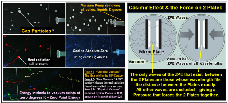
Figure 6: (Left) - Three Concepts of a Vacuum, Starting with A Perfectly Sealable Flask…. (Right) - an Experiment with Two Metal Plates in the Flask Which Shows a Vacuum Energy Exists as the Plates are Forced Together by Zpe Waves.
At this point, we get involved in a scientific mix-up or wrong turning which is stll influencing scientific opinions today. It also colors our outlook as to what a vacuum is. Please bear with us as we sort this through. In his first paper of 1901, Max Planck had arbitrarily inserted the factor “h” into his radiation equations. This factor had no actual physical significance in this first paper [20]. Although this mathematical manoeuver achieved the right answer, this situation was unsatisfactory to Planck. After due consideration, he corrected this defect in his second paper of 1911 [18]. In that paper, his equations revealed the existence of the ZPE, and the quantity “h” turned out to be a measure of the ZPE strength. So, on Planck’s new approach, “h” had a physical signifcance, namely an energy intrinsic to the vacuum. Furthermore, his equations showed that this vacuum energy was entirely independent of temperature. In 1916, Einstein and Nernst followed through with a paper which showed that this vacuum energy must also be all-pervasive and universal [21].
Although there was discussion about this concept into the early 1920’s, the situation changed in the period 1923 to 1927 when 4 papers were formulated and presented based on Planck’s 1st paper [22]. Because “h” had no physical meaning in Planck’s 1st paper, its effects in the equations in these resulting 4 papers could only be construed as being due to a strange property of atomic or sub-atomic matter itself, without any outside influence. However, these 4 papers followed Planck’s 1st paper, and the resulting intense discussion set the direction that this branch of physics was to follow for some time.
This contrasts sharply with Planck’s 2nd paper, in which “h” was a measure of ZPE strength. That means that whenever “h” appeared in the resulting equations, the effects were being caused by the outside action of the ZPE on sub-atomic matter, rather than any strange property of atomic matter itself.
It was in the middle of the intense disussion of those 4 papers, that Robert Mulliken presented his experimental results. He had essentially proved that the vacuum energy of Planck’s 2nd paper really existed. He found that the spectral lines emitted by boron monoxide had wavelengths shifted from their theoretical position by the action of the vacuum ZPE [19].
While some saw this result in these terms, and therefore a confirmation of the correctness of Planck’s 2nd paper, the success of the discussions about the 4 papers just presented induced many to interpret these results in a different way. Those 4 papers had led scientists to accept the idea that the ZPE was only a virtual concept, not real entity. They considered it was a mathematical abstraction which, for some purposes, was considered infinite, while at other times could be relegated to zero. So Mulliken’s results were sidelined. This continued until 1947 when the experiments of Willis Lamb produced very similar shifts in the spectral lines from hydrogen atoms to those seen by Mulliken. The effect has been known as the Lamb shift ever since [23].
As a result of this 1947 discovery, the Dutch scientist, Hendrik Casimir theorized in 1948 that it should be possible to test whether the ZPE was real or only virtual by an experimental arrangement now called the Casimir effect [24]. The effect verified the existence of a real ZPE when the experiment was conducted by M.J. Sparnaay 9 years later in Phillips Laboratories, Eindhoven, Holland in 1957 and reported in 1958 [25]. This experimental arrangement is sketched on the right hand segment of Figure 6 above. Our insulated and cold vacuum now has two metal plates as well as a device to measure the forces acting on those plates. The basis of the experiment is standard electromagnetcs, which says that any radiation that exists between such metal plates must have a wavelength, or multiple wavelengths, which fit exactly between the plates. If there is a real (not virtual) ZPE within the vacuum, there will be many different wavelengths throughout the flask. However, all those wavelengths which do not fit exactly between the plates will be excluded. This leads to an external pressure excess from all the excluded, longer waves, which will tend to collapse the plates as shown in Figure 6 on the right hand section.
While this experiment in 1957 proved there indeed was a variety of wavelengths in the flask near zero K, a strict theoretical analysis indicated that, if these results really came from a vacuum ZPE and not some other possible source, the Casimir effect should be directly proportional to the area of the plates. However, unlike all other forces with which it may be confused, the Casimir force tending to push the plates together must be inversely proportional to the fourth power of the plate’s distance apart. An experiment was thus still needed to prove that it was indeed a vacuum ZPE that was producing the results and not some other cause. If it was some other cause, the standard explanation of a virtual ZPE could still hold. It was not untl 40 years later that technology had advanced enough to make this experiment possible. In January of 1997, Steven Lamoreaux reported experimental verification of these predictions about the Casimir effect and the Casimir force to within 5% [26]. Then in November 1998, Umar Mohideen and Anushree Roy reported verification to within 1% in an experiment utilizing an atomic force microscope [27]. Planck’s theoretical proposal of the existence of the ZPE and its temperature independence, which only emerged in his second paper of 1911, had finally been verified, and Mulliken’s experimental proof vindicated as belonging to a real ZPE [18].
Although many physicsts did little to alter their stance on the ZPE after the 1957 results, those results set Louis de Broglie thinking. He had written the opening paper of the 4 which brought about the changed outlook in physics in the 1920’s [22]. Now, in 1962, he wondered if physics had missed a key ingredient by ignoring the effects of a real, not virtual, ZPE on atoms and subatomic particles. He published a book that year which started a re-examination of the alternative approach using a real ZPE as an agent in atomic behavior [28]. First, in 1966, Edward Nelson published a landmark paper deriving the Schroedinger equation from classical physics using the action of a real ZPE on particles of matter in a manner similar to Brownian motion [29]. Then in 1975, Timothy Boyer, using classical physics plus a real ZPE demonstrated that the continual battering of the ZPE waves produced exactly the same uncertainty in position and momentum at any instant as the Heisenberg Uncertainty Princple required [30]. That showed the ZPE wave impacts cause an electron to oscillate at the Compton frequency, namely 1.23 x 10^20 hits per second [31]. The physical reality of this was verified in an experiment using calcium ions by Gerritsma, Roos and colleagues in 2010 [32]. Then an analysis by Bernard Haisch and Alfonso Rueda demonstrated that, when the Compton frequency jitter is combined with the motion of an electron, there is a beat frequency superimposed on the oscillation which proves to be exactly the same as the de Broglie wavelength [31].
So, essentially, it has only been since 1998, and finally in 2010, that the theoretical and physical evidence has shown unequivocally that a real, all-pervasive ZPE exists. This, then, explains atomic phenomena logically. All that is needed is simple mathematics dealing with reality rather than some virtual idea. As a result, the option of a real cosmological ZPE is preferred here and will be used in the rest of this paper. In fact, there are three key matters needing explanation here on this new understanding of the ZPE. First is the link between the ZPE and atomic masses; second is the role of the ZPE in atomic stability; and third is the origin of the ZPE itself. Let us look briefly at these and then see how this impacts our study of the redshift.
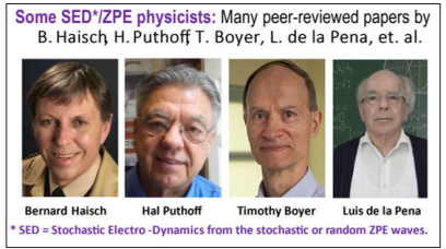
Figure 7: Some of the 200 or so Active ZPE Physicists
Many modern theories envisage sub-atomic particles (which Richard Feynman referred to as “partons”) making up matter as being charged point particles with a form, but no intrinsic mass. This concept originated with a long line of investigators, including Planck and Einstein, who developed radiation theory on the basis of the behavior of mass-less, charged, point particle oscillators. Since the resulting radiation theory was in agreement with the data, the problem was to understand how mass was imparted to these mass-less oscillators, and hence to all matter, by physicists who hold to a virtual ZPE. Eventually, the Higgs boson was postulated to do the job, even though problems still persist with that model.
In contrast, ZPE physicists note that the electromagnetic waves of the ZPE impinge on all the charged mass-less particles, which causes them to “jitter” either at, or very close to the speed of light. This conclusion has been sustained by recent studies and the term “ultra-relativistic” has been used to descrbe it [33, 34]. ZPE physicst Hal Puthoff explains what happens using this approach: “In this view, the particle mass, m, is of dynamical origin, originating in the parton-motion response to the electromagnetic zeropoint fluctuations of the vacuum. It is therefore simply a special case of the general proposition that the internal kinetic energy of a system contributes to the effective mass of that system” [35]. As a result it was then stated that even if it was found to exist, “the Higgs might not be needed to explain rest mass at all. The inherent energy in a particle may be a result of its jittering motion [caused by the ZPE]. A massless particle may pick up energy from it [the ZPE], hence acquiring what we think of as rest mass” [36]. The calculations of these ZPE physicists quantitatively support this view [35, 37]. In summary, the impacting waves of the ZPE on sub-atomic particles cause them to move close to the speed of light. This is a kinetic energy which, because of the equivalence of mass and energy, gives an intrinsic mass to these partons.
A problem presented by classical physics is that an electron orbiting a proton or atomic nucleus will be radiating energy. As a result, as the electron loses energy, it should spiral into the nucleus and the atom disappear in a flash of light. This does not happen, and many physicists answer the problem by invoking quantum laws, implying that matter simply behaves that way as one of its strange intrinsic properties. However, it would seem to be preferable to have an actual physical explanation if we could find one.
According to ZPE physicists, classical physics is indeed correct when it considers electrons to be radiating energy as it circles the nucleus. However, this energy loss must be coupled with the energy absorbed from the ZPE. Quantitative analyses were done and the results summarized by de la Pena who stated that: “Boyer and Claverie & Diner have shown that if one considers circular orbits only, then one obtains an equilibrium [orbit] radius of the expected size [the Bohr radius]: for smaller distances, the electron absorbs too much energy from the [ZPE] field…and tends to escape, whereas for larger distances it radiates too much and tends to fall towards the nucleus” [30, 38, 39].
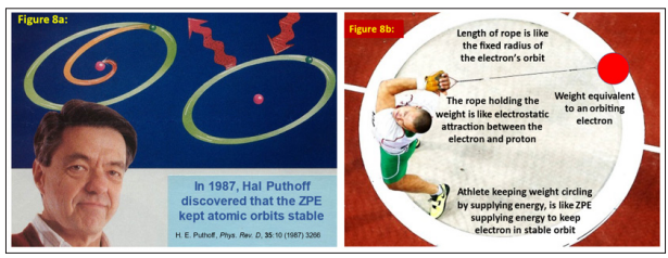
In 1987, Hal Puthoff examined the situation further in this ZPE context. His conclusion carries unusual significance. It reads: “Finally, it is seen that a well-defined, precise quantitative argument can be made that the ground state of the hydrogen atom is defined by a dynamic equilibrium in which the collapse of the state is prevented by the presence of the zero-point fluctuations of the electromagnetic field. This carries with it the attendant implication that the stability of matter itself is largely mediated by the ZPF phenomena in the manner described here, a concept that transcends the usual interpretation of the role and significance of zero-point fluctuations of the vacuum electromagnetic field” [40]. Note that “ZPF” here refers to “zero-point fields” or “zeropoint fluctuations.”
Thus the very existence of atomic structures depends on this allpervasive ZPE sea. Without it, all matter in the cosmos collapses. New Scientist discussed this in July 1987 and July 1990 under the heading “Why atoms don’t collapse.” See Figure 8a as an illustration of what is happening. Puthoff’s analysis showed that energy may be considered as being fed into the orbiting electron via the angular momentum, which is governed by Planck’s constant “h,” or multiples thereof, in the usual equations. This is logical as “h” is a measure of the strength of the ZPE which determines atomic behavior.
To understand this in a very simplified way using the angular momentum aproach, consider Figure 8b. There the athlete is swinging a weight around in a circle. The athlete has to expend energy to keep the weight moving in a circle. Imagine that the weight at the end of the rope is an electron, and the fixed length of rope is the radius of the electron’s orbit. For an atom, the rope is the electrical attraction between the electron and the proton. The action of the athlete keeping the weight circling about him is equivalent to the ZPE keeping the electron moving in a stable orbit and not letting it slow down. We will return to this aspect of the topic in a moment.
The third matter requiring explanation is the origin of the ZPE itself. This involves a concept sometimes called the “fabric of space,” which hints that some sort of “structure” to the vacuum exists, rather like the weave in the fabric of a cloth. The fabric of space is considered by some scientists to be made up of a “weave” of particles. The exact nature of these particles is debated. String theorists consider them to be extra dimensions rolled up into strange ball-like Calabi-Yau shapes. Others consider the “weave” to be made up of spinning, but oppositely-charged particle pairs which have intrinsic electric and magnetic fields. Some consider the magnetic fields to arise because of all the movement of these charged particles. Their opposite charges maintain vacuum neutrality. The particles or shapes themselves are called Planck particles or Planck particle pairs.
As the expansion or stretching of space went on at its most basic level, the fabric of space was being stretched also. This means the Planck particles were being pulled apart. Today, it is considered that the separation of these particle is about 10^ -35 meters, (called the Planck length), and this resulted in a tension or force being manifest between the particles. The resulting electromagnetic energy is called the Zero Point energy. Furthermore, as the expansion continued, the ZPE continued to build up. Gibson has shown in detail how this expansion generates cascades of more Planck particle pairs whose numbers will increase as the expansion goes on [41]. Hoyle, Burbidge and Narlikar have a different mechanism but it essentially produces the same result [42]. The turbulent gyrations of these particles would radiate electromagnetic energy into their environment. Effectively this means that the ZPE will continue to build with cosmic expansion. Finally, ZPE physicists have shown how, once it was established, the ZPE will be maintained by a “self-regenerating feedback cycle” [43].
The fact that the Zero Point Energy has increased as universal expansion has continued opens up some new scenarios on a range of scientific topics, some of which are explored in this Conference Monograph [44]. However, this present paper is particularly interested in the consequences for some specific atomic behavior.
First, an increasing ZPE means an increasing value for Planck’s constant, “h,” since Planck’s equations in his 2nd paper revealed that “h” was a measure of the strength of the ZPE. In turn, this would mean that there are more hits per second on sub-atomic particles, like electrons. This results in a greater jitter per second, which in turn means an increase in particle kinetic energy. Consequently, the rest-masses, “m,” of all sub-atomic particles must increase as well.
Second, this joint increase in Planck’s constant, “h”, and particle rest-masses, “m”, means that atomic orbit energies will also increase, even though orbit radii remain fixed. In turn, that means that the light emitted from atoms will become progressively more energetic and hence move towards the blue end of the spectrum with time. Therefore, as we look progressively farther out into space and so further back in time, the light emitted by atoms in those distant galaxies wlll be increasingly redder than now. Therefore, the redhift of light from distant galaxies may not be because of a Doppler shift or becase of light waves being stretched by expansion, but rather because the ZPE strength was systematically lower in the earlier universe.
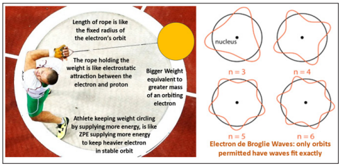
Figure 9: Analogies of electron orbit behavior with increasing ZPE strength
There is one additional factor in all this. Electrons can only circle the nucleus in orbits which accommodate their de Broglie waves (or their multiples) exactly as in the right hand segment of Figure 9.The waves may have varying numbers of “nodes” but they all fit the orbit exactly. If they did not, the waves would cancel out. Therefore, as the ZPE builds up and atomic masses increase, orbit energy also increases. However, no change in the emitted light will occur, until the energy builds up sufficently for the wave pattern to jump to the next node number. Since the orbit wave pattern governs the wavelength of the emitted light, then, as the ZPE strength smoothly increases, the emitted light will become bluer, not smoothly, but in jumps; that is to say, it is quantized. In order for this scenario to be fulfilled, analysis indicates that the necessary condition is that the orbit velocity, v is proportional to the cube-root of 1 / (h^2). However, the logical proof of this takes more time and space than we have in this paper.
This ZPE approach therefore gives a different reason for the redshift, which is still indirectly caused by universal expansion. In addition, it explains why the redshift may be quantized. Finally, it makes it possible for the observed redshift of some groups of objects to actually become less by one qantum jump as the ZPE strength increases and emitted light becomes bluer by one jump. The implications of these studies opens up a whole range of potentially fruitful research.