Author(s): Gerald C Hsu
Recently, the author applied theories of viscoelasticity and viscoplasticity from engineering and perturbation theory from quantum mechanics to conduct his biomedical research on output biomarkers of cancer risk probability percentage (symptoms or behaviors) resulting from suspected or identified input biomarkers of lifestyle scores (causes or stressors). The lifestyle scores are calculated as a combination of his individual performance level for food, diet, exercise, sleep, stress, water intake, and daily life routines. His developed lifestyle model includes key environmental factors such as air and water pollution, nuclear radiation, toxic chemical exposure, food poisoning, and hormone therapy along with life-long bad habits, such as drinking alcohol, smoking cigarettes, and illicit drug use. For the author himself, he has no bad habits and has limited environmental exposure.
In this particular article, he studies the correlation between his cancer Risk % versus his lifestyle scores. He then applies the viscoelastic or viscoplastic glucose theory (VGT) to construct a stress-strain diagram to verify the existing time-dependency characters of both input biomarker (lifestyle score) and output biomarker (cancer Risk %). Finally, he utilizes the visco-perturbation model and lifestyle score alone to predict his cancer risk probability % to compare against his calculated cancer risk probability % using his developed metabolism index (MI) model. Out of curiosity, he further investigates the relationship between cancer risk % and diabetic glucose level to explore the strength of inter-relationship between symptoms for two diseases, cancer versus diabetes, not between root-cause and symptom. The timeframe of this study covers a long period of 10+ years from Y2012 to Y2022.
The following two defined equations from viscoelasticity or viscoplasticity are utilized to study the stress-strain relationship in his cases. Here, he wants to use the strain rate or his annual cancer risk change rate multiplied with the viscosity factor, lifestyle score, as the stress:
strain = ε
= individual output biomarker value (cancer risk %) at present time
Stress = σ
= η * (dε/dt)
= η * (d-strain/d-time)
= (viscosity factor η, i.e. lifestyle score) * ((output biomarker of cancer risk at present time - output biomarker of cancer risk at previous time) / (time duration = 1))
Where the time duration of 1 was chosen due to his annual cancer risk probability % taken at 1-year intervals. After completing the steps from above, he generated the following four useful information:
(1) An organized data table which contains the input biomarker (viscosity factor η, lifestyle score) and output biomarker (cancer risk %) to construct a time-domain (TD) waveform diagram.
(2) A constructed stress-strain diagram in space-domain (SD) using the strain rate (dε/dt), annual cancer risk changing rate, multiplied with the viscosity factor η (annual lifestyle score i.e., input biomarker), as the stress. This calculated annual cancer risk probability % is the strain.
(3) A calculation of prediction accuracy and waveform similarity through the correlation coefficient between calculated cancer risk based on MI and predicted cancer risk based on the visco-perturbation model.
(4) An extra correlation study between cancer risk and diabetic glucose (estimated daily glucose or eAG).
To offer a simple explanation to readers who do not have a physics or engineering background, the author includes a brief excerpt from Wikipedia regarding the description of basic concepts for elasticity and plasticity theories, viscoelasticity and viscoplasticity theories from the disciplines of engineering and physics, along with perturbation theory of quantum mechanics in the Method section.
In summary, the following five observations outline the findings from this research work.
(1) From the TD analysis, the waveforms of his calculated overall cancer risk probability and his measured lifestyle score are high with a 96% correlation. It should be noted that the lifestyle score is the input biomarker while the cancer risk is the output biomarker.
(2) In contrast, from another TD analysis, the waveforms of his calculated overall cancer risk probability % and his measured glucose value (eAG) are also high with an 81% correlation but not as high as 96% of the much closer relationship between the cancer risk as to the symptom and the lifestyle score as the root cause. It should be noted that both glucose (eAG) values of diabetes and cancer risk % are the output symptoms.
(3)“Overall, only 8%-18% of cancer patients have diabetes. In the context of epidemiology, the burden of both diseases, and the small association between them will be clinically relevant and should translate into significant consequences for future healthcare solutions. People with diabetes are at increased risk for cancer. The risk is highest for liver, pancreatic, colorectal, endometrial, breast, and bladder cancer. People with type 2 diabetes (T2D) are twice as likely to develop liver or pancreatic cancer.” The above excerpts are quoted from Hindawi and MD Anderson.
(4) The stress-strain diagram of cancer risk versus cancer change rate multiplied by the lifestyle score demonstrates the viscoplastic characteristics, or time-dependency, of the two biomarkers.
(5) Regarding the comparison between the predicted cancer risk utilizing the visco-perturbation model and the calculated cancer risk using the MI model, they depict an extremely high correlation of 98% along with the prediction accuracy of 98% as well.
In conclusion, utilizing the VGT in combination with the perturbation model can provide a practical and accurate predicted cancer risk probability % using lifestyle score as the influential factor. In addition, this study has shown a very high correlation between cancer risk as to the symptom and lifestyle score as the root cause. However, when he compares the symptoms of these two diseases, cancer and diabetes, the correlation between these two symptoms is not as high as the correlation between the symptom and the root cause of cancer.
Keyword: Geriatric, Cancer & Dementia
Recently, the author applied theories of viscoelasticity and viscoplasticity from engineering and perturbation theory from quantum mechanics to conduct his biomedical research on output biomarkers of cancer risk probability percentage (symptoms or behaviors) resulting from suspected or identified input biomarkers of lifestyle scores (causes or stressors). The lifestyle scores are calculated as a combination of his individual performance level for food, diet, exercise, sleep, stress, water intake, and daily life routines. His developed lifestyle model includes key environmental factors such as air and water pollution, nuclear radiation, toxic chemical exposure, food poisoning, and hormone therapy along with life-long bad habits, such as drinking alcohol, smoking cigarettes, and illicit drug use. The author himself has no bad habits and has limited environmental exposure.
In this particular article, he studies the correlation between his cancer Risk % versus his lifestyle scores. He then applies the viscoelastic or viscoplastic glucose theory (VGT) to construct a stress-strain diagram to verify the existing time-dependency characteristics of both input biomarker (lifestyle score) and output biomarker (cancer Risk %). Finally, he utilizes the visco perturbation model and lifestyle score alone to predict his cancer risk probability % to compare against his calculated cancer risk probability % using his developed metabolism index (MI) model. Out of curiosity, he further investigates the relationship between cancer risk % and diabetic glucose level to explore the strength of the inter-relationship between symptoms for two diseases, cancer versus diabetes, not between root cause and symptom. The timeframe of this study covers a long period of 10+ years from Y2012 to Y2022.
The following two defined equations from viscoelasticity or viscoplasticity are utilized to study the stress-strain relationship in his cases. Here, he wants to use the strain rate or his annual cancer risk change rate multiplied by the viscosity factor, and lifestyle score, as the stress:
Where the time duration of 1 was chosen due to his annual cancer risk probability % taken at 1-year intervals.
After completing the steps from above, he generated the following four useful information:
To offer a simple explanation to readers who do not have a physics or engineering background, the author includes a brief excerpt from Wikipedia regarding the description of basic concepts for elasticity and plasticity theories, viscoelasticity and viscoplasticity theories from the disciplines of engineering and physics, along with perturbation theory of quantum mechanics in the Method section.
In the author’ s published paper No.484: “Estimated relative cancer risks using metabolism index model, including weighted lifestyle scores and certain metabolic biomarker values from a collected 7-years big data of a type 2 diabetes patient based on GH-Method: math-physical medicine (No. 484)” written on 7/21-29/2021, he wrote his findings and personal feelings below, after reading the Reviews/Commentaries/ADA Statements, “Diabetes and Cancer, A consensus report” by Edward Giovannucci, MD, and other authors, published by the American Diabetes Association and the American Cancer Society.
“In the consensus report on diabetes and cancers, the original paper’ s authors have repetitively used the phrases like: “lacking epidemiological evidence, having incomplete biological links, or facing unclear pathophysiologies underlying the association between diabetes and cancers directly”. This has caused the author of this article to think about the meaning of this subject deeper using his physics and engineering background.
Even though various cancers have their different causes and diabetes has its specific causes, the majority of these two families of disease causes are overlapping with each other. To identify the direct relationship between diabetes and cancers based on symptoms which is more unclear or even difficult, it may be easier to start with the digging into their overlapping causes (around 70% to 80% of causes are overlapping), e.g. lifestyle, life-long bad habits, environmental factors, such as a toxin, pollution, radiation, etc., and overall metabolism.
This situation can be illustrated using the author’ s engineering and physics background. The tensile stress (stretching force) and strain (longitudinal deformation) are dependent on Young’ s modulus,while the shear stress (shear force) and strain (shear deformation) are dependent on the shear modulus. However, both Young’ s modulus (similar to cancer’ s relationship between its causes and symptoms) and shear modules (similar to the diabetes relationship between its causes and symptoms) are directly related to the actual material of the study subject. The engineering material (or human body) contains both Young’ s modulus and shear modulus which is similar to our human body is under the influences of common causes, such as life habits, lifestyle details, environmental factors, and metabolism. Therefore, we better start with the understanding of the material first (i.e. the underlying causes), instead of directly searching for the relationship between those vast numbers of symptoms of diseases of cancers and diabetes.”
The author has collected ~3 million data regarding his health condition and lifestyle details over the past 12 years. He spent the entire year of 2014 developing a metabolism index (MI) model using topology concept, nonlinear algebra, algebraic geometry, and finite element method. This MI model contains various measured biomarkers and recorded lifestyle details along with their induced new biomedical variables for an additional ~1.5 million data. Detailed data of his body weight, glucose, blood pressure, heart rate, blood lipids, body temperature, and blood oxygen level, along with important lifestyle details, including diet, exercise, sleep, stress, water intake, and daily life routines are included in his MI database. In addition, these lifestyle details also include some lifetime bad habits and environmental exposures. Luckily, the author has none of these lifetime bad habits and also with a very low degree of exposure to those environmental factors. His developed MI model has a total of 10 categories covering approximately 500 detailed elements that constitute his defined “metabolism model” which are the building blocks or root causes for diabetes and other chronic disease complications, including but not limited to cardiovascular disease (CVD), chronic heart disease (CHD), stroke, chronic kidney disease (CKD), retinopathy, neuropathy, foot ulcer, and hypothyroidism. The end result of the MI development work is a combined MI value within any selected time period with 73.5% as its dividing line between a healthy and unhealthy state. The MI serves as the foundation to many of his follow-up medical research work.
During the period from 2015 to 2017, he focused his research on type 2 diabetes (T2D), especially glucoses, including fasting plasma glucose (FPG), postprandial plasma glucose (PPG), estimated average glucose (eAG), and hemoglobin A1C (HbA1C). During the following period from 2018 to 2022, he concentrated on researching medical complications resulting from diabetes, chronic diseases, and metabolic disorders which include heart problems, stroke, kidney problems, retinopathy, neuropathy, foot ulcer, diabetic skin fungal infection, hypothyroidism, and diabetic constipation, cancer, and dementia. He also developed a few mathematical risk models to calculate the probability percentages of developing various diabetic complications.
From his previous medical research work, he has identified and learned that those associated energy of hyperglycemia conditions are the primary source of causing many diabetic complications which lead to death. Therefore, a thorough knowledge of these energies is important for achieving a better understanding of those dangerous complications.
(from “Soborthans, innovating shock and vibration solutions”)
Elasticity is the tendency of solid materials to return to their original shape after forces are applied on them. When the forces are removed, the object will return to its initial shape and size if the material is elastic.
Viscosity is a measure of a fluid’ s resistance to flow. A fluid with large viscosity resists motion. A fluid with low viscosity flows. For example, water flows more easily than syrup because it has a lower viscosity. High viscosity materials might include honey, syrups, or gels - generally, things that resist flow. Water is a low viscosity material, as it flows readily. Viscous materials are thick or sticky or adhesive. Since heating reduces viscosity, these materials don’ t flow easily. For example, warm syrup flows more easily than cold.
Viscoelasticity is the property of materials that exhibit both viscous and elastic characteristics when undergoing deformation. Synthetic polymers, wood, and human tissue, as well as metals at high temperature, display significant viscoelastic effects. In some applications, even a small viscoelastic response can be significant.
The difference between elastic materials and viscoelastic materials is that viscoelastic materials have a viscosity factor and the elastic ones don’ t. Because viscoelastic materials have the viscosity factor, they have a strain rate dependent on time. Purely elastic materials do not dissipate energy (heat) when a load is applied, then removed; however, a viscoelastic substance does.
The physical property is when materials or objects return to their original shape after deformation
In physics and materials science, elasticity is the ability of a body to resist a distorting influence and to return to its original size and shape when that influence or force is removed. Solid objects will deform when adequate loads are applied to them; if the material is elastic, the object will return to its initial shape and size after removal. This is in contrast to plasticity, in which the object fails to do so and instead remains in its deformed state.
The physical reasons for elastic behavior can be quite different for different materials. In metals, the atomic lattice changes size and shape when forces are applied (energy is added to the system). When forces are removed, the lattice goes back to the original lower energy state. For rubbers and other polymers, elasticity is caused by the stretching of polymer chains when forces are applied.
Hooke’ s law states that the force required to deform elastic objects should be directly proportional to the distance of deformation, regardless of how large that distance becomes. This is known as perfect elasticity, in which a given object will return to its original shape no matter how strongly it is deformed. This is an ideal concept only; most materials that possess elasticity in practice remain purely elastic only up to very small deformations, after which plastic (permanent) deformation occurs.
In engineering, the elasticity of a material is quantified by the elastic modulus such as Young’ s modulus, bulk modulus, or shear modulus which measure the amount of stress needed to achieve a unit of strain; a higher modulus indicates that the material is harder to deform. The material’ s elastic limit or yield strength is the maximum stress that can arise before the onset of plastic deformation.
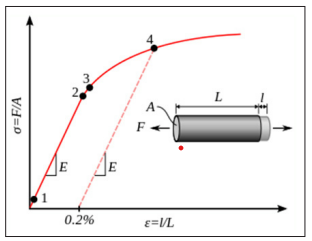
Deformation of a solid material undergoing non-reversible changes of shape in response to applied forces.
In physics and materials science, plasticity, also known as plastic deformation, is the ability of a solid material to undergo permanent deformation, a non-reversible change of shape in response to applied forces. For example, a solid piece of metal being bent or pounded into a new shape displays plasticity as permanent changes occur within the material itself. In engineering, the transition from elastic behavior to plastic behavior is known as yielding.
Stress-strain curve showing typical yield behavior for nonferrous
alloys.
1. True elastic limit
2. Proportionality limit
3. Elastic limit
4. Offset yield strength
A stress-strain curve typical of structural steel.
Plastic deformation is observed in most materials, particularly metals, soils, rocks, concrete, and foams. However, the physical mechanisms that cause plastic deformation can vary widely. At a crystalline scale, plasticity in metals is usually a consequence of dislocations. Such defects are relatively rare in most crystalline materials, but are numerous in some and part of their crystal structure; in such cases, plastic crystallinity can result. In brittle materials such as rock, concrete and bone, plasticity is caused predominantly by slip at microcracks. In cellular materials such as liquid foams or biological tissues, plasticity is mainly a consequence of bubble or cell rearrangements, notably T1 processes.
For many ductile metals, tensile loading applied to a sample will cause it to behave in an elastic manner. Each increment of load is accompanied by a proportional increment in extension. When the load is removed, the piece returns to its original size. However, once the load exceeds a threshold - the yield strength - the extension increases more rapidly than in the elastic region; now when the load is removed, some degree of extension will remain.
Elastic deformation, however, is an approximation and its quality depends on the time frame considered and loading speed. If, as indicated in the graph opposite, the deformation includes elastic deformation, it is also often referred to as “elasto-plastic deformation” or “elastic-plastic deformation”.
Perfect plasticity is a property of materials to undergo irreversible deformation without any increase in stresses or loads. Plastic materials that have been hardened by prior deformation, such as cold forming, may need increasingly higher stresses to deform further. Generally, plastic deformation is also dependent on the deformation speed, i.e. higher stresses usually have to be applied to increase the rate of deformation. Such materials are said to deform visco-plastically.”
Property of materials with both viscous and elastic characteristics under deformation
In materials science and continuum mechanics, viscoelasticity is the property of materials that exhibit both viscous and elastic characteristics when undergoing deformation. Viscous materials, like water, resist shear flow and strain linearly with time when a stress is applied. Elastic materials strain when stretched and immediately return to their original state once the stress is removed.
Viscoelastic materials have elements of both of these properties and, as such, exhibit time-dependent strain. Whereas elasticity is usually the result of bond stretching along crystallographic planes in an ordered solid, viscosity is the result of the diffusion of atoms or molecules inside an amorphous material.
In the nineteenth century, physicists such as Maxwell, Boltzmann, and Kelvin researched and experimented with creep and recovery of glasses, metals, and rubbers. Viscoelasticity was further examined in the late twentieth century when synthetic polymers were engineered and used in a variety of applications. Viscoelasticity calculations depend heavily on the viscosity variable, η. The inverse of η is also known as fluidity, Φ. The value of either can be derived as a function of temperature or as a given value (i.e. for a dashpot).
Depending on the change of strain rate versus stress inside a material, the viscosity can be categorized as having a linear, non-linear, or plastic response. When a material exhibits a linear response it is categorized as a Newtonian material. In this case the stress is linearly proportional to the strain rate. If the material exhibits a non-linear response to the strain rate, it is categorized as Non-Newtonian fluid. There is also an interesting case where the viscosity decreases as the shear/strain rate remains constant. A material which exhibits this type of behavior is known as thixotropic. In addition, when the stress is independent of this strain rate, the material exhibits plastic deformation. Many viscoelastic materials exhibit rubber like behavior explained by the thermodynamic theory of polymer elasticity.
Cracking occurs when the strain is applied quickly and outside of the elastic limit. Ligaments and tendons are viscoelastic, so the extent of the potential damage to them depends both on the rate of the change of their length as well as on the force applied.
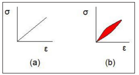
Stress-strain curves for a purely elastic material (a) and a viscoelastic material (b). The red area is a hysteresis loop and shows the amount of energy lost (as heat) in a loading and unloading cycle. It is equal to
Φσdε
where σ is stress and ε is strain.
Unlike purely elastic substances, a viscoelastic substance has an elastic component and a viscous component. The viscosity of a viscoelastic substance gives the substance a strain rate dependence on time. Purely elastic materials do not dissipate energy (heat) when a load is applied, then removed. However, a viscoelastic substance dissipates energy when a load is applied, then removed. Hysteresis is observed in the stress-strain curve, with the area of the loop being equal to the energy lost during the loading cycle. Since viscosity is the resistance to thermally activated plastic deformation, a viscous material will lose energy through a loading cycle. Plastic deformation results in lost energy, which is uncharacteristic of a purely elastic material’ s reaction to a loading cycle.
Specifically, viscoelasticity is a molecular rearrangement. When a stress is applied to a viscoelastic material such as a polymer, parts of the long polymer chain change positions. This movement or rearrangement is called “creep”. Polymers remain a solid material even when these parts of their chains are rearranging in order to accompany the stress, and as this occurs, it creates a back stress in the material. When the back stress is the same magnitude as the applied stress, the material no longer creeps. When the original stress is taken away, the accumulated back stresses will cause the polymer to return to its original form. The material creeps, which gives the prefix visco-, and the material fully recovers, which gives the suffix -elasticity.
Viscoplasticity is a theory in continuum mechanics that describes the rate-dependent inelastic behavior of solids. Rate-dependence in this context means that the deformation of the material depends on the rate at which loads are applied. The inelastic behavior that is the subject of viscoplasticity is plastic deformation which means that the material undergoes unrecoverable deformations when a load level is reached. Rate-dependent plasticity is important for transient plasticity calculations. The main difference between rate independent plastic and viscoplastic material models is that the latter exhibit not only permanent deformations after the application of loads but continue to undergo a creep flow as a function of time under the influence of the applied load.
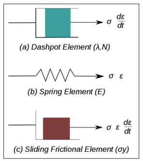
Figure 1: Elements used in One-Dimensional Models of Viscoplastic Materials
The elastic response of viscoplastic materials can be represented in one dimension by Hookean spring elements. Rate-dependence can be represented by nonlinear dashpot elements in a manner similar to viscoelasticity. Plasticity can be accounted for by adding sliding frictional elements as shown in Figure 1. In figure B is the modulus of elasticity, λ is the viscosity parameter and N is a power-law type parameter that represents non-linear dashpot [σ(dε /dt)= σ = λ(dε /dt)(1/N)]. The sliding element can have a yield stress (σy) that is strain rate dependent, or even constant, as shown in Figure 1c.
Viscoplasticity is usually modeled in three dimensions using overstress models of the Perzyna or Duvaut-Lions types. In these models, the stress is allowed to increase beyond the rate independent yield surface upon application of a load and then allowed to relax back to the yield surface over time. The yield surface is usually assumed not to be rate-dependent in such models. An alternative approach is to add a strain rate dependence to the yield stress and use the techniques of rate independent plasticity to calculate the response of a material.
For metals and alloys, viscoplasticity is the macroscopic behavior caused by a mechanism linked to the movement of dislocations in grains, with superposed effects of inter-crystalline gliding. The mechanism usually becomes dominant at temperatures greater than approximately one third of the absolute melting temperature. However, certain alloys exhibit viscoplasticity at room temperature (300K). For polymers, wood, and bitumen, the theory of viscoplasticity is required to describe behavior beyond the limit of elasticity or viscoelasticity.
In general, viscoplasticity theories are useful in areas such as
For a qualitative analysis, several characteristic tests are performed
to describe the phenomenology of viscoplastic materials. Some
examples of these tests are
1. hardening tests at constant stress or strain rate,
2. creep tests at constant force, and
3. stress relaxation at constant elongation.
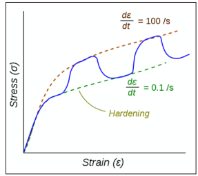
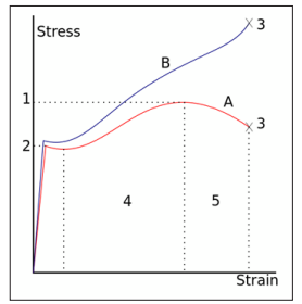
Figure 2: Stress-Strain Response of a Viscoplastic Material at Different Strain Rates.
The dotted lines show the response if the strain-rate is held constant. The blue line shows the response when the strain rate is changed suddenly.
One consequence of yielding is that as plastic deformation proceeds, an increase in stress is required to produce additional strain. This phenomenon is known as Strain/Work hardening. For a viscoplastic material the hardening curves are not significantly different from those of rate-independent plastic material. Nevertheless, three essential differences can be observed.
1. At the same strain, the higher the rate of strain the higher
the stress
2. A change in the rate of strain during the test results in an
immediate change in the stress-strain curve.
3. The concept of a plastic yield limit is no longer strictly
applicable
The hypothesis of partitioning the strains by decoupling the elastic and plastic parts is still applicable where the strains are small, i.e.,
ε = ε e + ε vp
where ε e is the elastic strain and ε vp is the viscoplastic strain. To obtain the stress-strain behavior shown in blue in the figure, the material is initially loaded at a strain rate of 0.1/s. The strain rate is then instantaneously raised to 100/s and held constant at that value for some time. At the end of that time period the strain rate is dropped instantaneously back to 0.1/s and the cycle is continued for increasing values of strain. There is clearly a lag between the strain-rate change and the stress response. This lag is modeled quite accurately by overstress models (such as the Perzyna model) but not by models of rate-independent plasticity that have a rate-dependent yield stress
This article is about perturbation theory as a general mathematical method. In mathematics and applied mathematics, perturbation theory comprises methods for finding an approximate solution to a problem, by starting from the exact solution of a related, simpler problem. A critical feature of the technique is a middle step that breaks the problem into “solvable” and “perturbative” parts. In perturbation theory, the solution is expressed as a power series in a small parameter ε . The first term is the known solution to the solvable problem. Successive terms in the series at higher powers of ε usually become smaller. An approximate ‘ perturbation solution’ is obtained by truncating the series, usually by keeping only the first two terms, the solution to the known problem and the ‘ first order’ perturbation correction.”
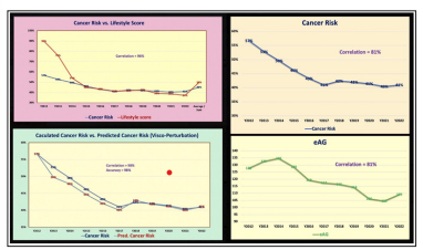
Figure 3 displays a data table of cancer risk, lifestyle score, visco perturbation calculation, and stress-strain data.
Figure 4 displays the annual cancer risk and annual lifestyle score from Y2012 to Y2022 in a time-domain (TD).
Figure 5 displays the stress-strain diagram in a frequency-domain (FD).
Figure 6 shows the comparison between calculated cancer risk using MI model and predicted cancer risk using visco-perturbation model. Both of their correlation and prediction accuracy are very high, at 98%.
Figure 7 provides a comparison between two symptoms, i.e. cancer and diabetes. Their correlation of 81% between two symptoms is lower than the correlation of 96% between cancer symptom and cancer cause.
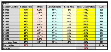
Figure 3: Data Table of Calculation
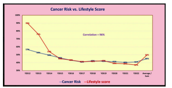
Figure 4: cancer risk % and lifestyle score waveforms in TD
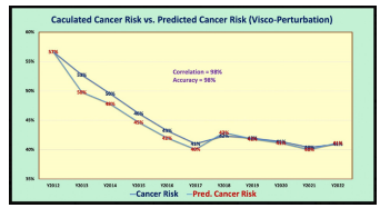
Figure 5: Stress-strain diagram in a spatial-domain (SD)
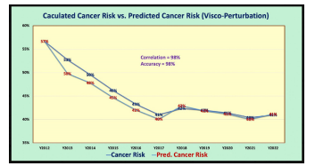
Figure 6: Calculated vs. Predicted cancer risk % in a time-domain (TD)
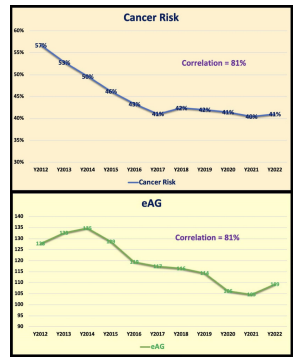
Figure 7: Comparison between cancer risk (symptom) and eAG of diabetes (symptom) with a lower 81% correlation
In summary, the following five observations outline the findings from this research work.
(1) From the TD analysis, the waveforms of his calculated overall cancer risk probability and his measured lifestyle score are high with a 96% correlation. It should be noted that the lifestyle score is the input biomarker while the cancer risk is the output biomarker.
(2) In contract, from another TD analysis, the waveforms of his calculated overall cancer risk probability % and his measured glucose value (eAG) are also high with an 81% correlation but not as high as 96% of the much closer relationship between the cancer risk as the symptom and the lifestyle score as the root-cause. It should be noted that both glucose (eAG) values of diabetes and cancer risk % are the output symptoms.
(3)“Overall, only 8%-18% of cancer patients have diabetes. In the context of epidemiology, the burden of both diseases, and the small association between them will be clinically relevant and should translate into significant consequences for future healthcare solutions. People with diabetes are at increased risk for cancer. The risk is highest for liver, pancreatic, colorectal, endometrial, breast, and bladder cancer. People with type 2 diabetes (T2D) are twice as likely to develop liver or pancreatic cancer.” The above excerpts are quoted from Hindawi and MD Anderson.
(4) The stress-strain diagram of cancer risk versus cancer change rate multiplied by the lifestyle score demonstrates the viscoplastic characteristics, or time-dependency, of the two biomarkers.
(5) Regarding the comparison between the predicted cancer risk utilizing the visco-perturbation model and the calculated cancer risk using the MI model, they depict an extremely high correlation of 98% along with the prediction accuracy of 98% as well.
In conclusion, utilizing the VGT in combination with the perturbation model can provide a practical and accurate predicted cancer risk probability % using lifestyle score as the influential factor. In addition, this study has shown a very high correlation between cancer risk as the symptom and lifestyle score as the root cause. However, when he compares the symptoms of these two diseases, cancer and diabetes, the correlation for these two symptoms are not as high as the correlation between the symptoms and root cause of cancer.
For editing purposes, the majority of the references in this paper, which are self-references, have been removed. Only references from other authors’ published sources remain. The bibliography of the author’ s original self-references can be viewed at www. eclairemd.com.
Readers may use this article as long as the work is properly cited, their use is educational and not for profit, and the author’ s original work is not altered.
View PDF